Common Method Bias in SEM Model

Over the last 10 years, more and more attention has been paid to the idea of common method bias (CMB) in the measurement analysis phase. Common method bias is the inflation (or in rare cases deflation) of the true correlation among observable variables in a study. Research has shown that because respondents are replying to survey questions about independent and dependent variables at the same time, this can artificially inflate the covariation (which lead to biased parameter estimates). Here are some ways to control for common method bias:

1. Harman’s Single Factor Test—this simplistic test performs an EFA with all the indicators in your model to determine if one single factor will emerge. If a single factor does appear, then common method bias is said to be present in the data.You will also see a Harman’s single factor test performed with a CFA where all indicators are purposely loaded on one factor to determine model fit. If you have an acceptable model fit with the one construct model, then you have a method bias.There is an ongoing debate as to whether Harman’s single factor test is an appropriate test to determine common method bias. On one side, researchers have questioned this approach and have concluded that it is insufficient to determine if common method bias is present (Malhotra et al. 2007; Chang et al. 2010). Other researchers (Fuller et al. 2016) have argued that if common method bias is strong enough to actually bias results, then Harman’s single factor test is sensitive enough to determine if a problem exists.While Harman’s single factor test is easy to implement, it is a relatively insensitive test to determine common method bias compared to other post- hoc tests. In my opinion, if you know a test is inferior to others, then there is very little justification for using this method.

2. Marker-Variable Technique—to use this test, the researcher has to plan ahead in the survey design phase of your This technique requires you to introduce a variable in a survey that is theoretically unrelated to any other construct in your study. This “mole” variable is also called the marker variable. CMB is assessed by examining the correlation between the marker variable and the unrelated variables of your study. Theoretically, the correlation between your marker variable and the variables of the study should be low. If the correlations are not low, there is a good chance you are going to have a significant method bias.To determine if this bias is present, you need to partial out the effect of the marker variable from all the correlations across constructs. In essence, you are going to strip out any inflated correlation because of a method bias from your other constructs.

Here is how to obtain the adjusted correlation between constructs with the marker variable’s influence removed:

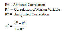
In the past, a researcher would use the lowest correlation of the marker variable and another construct in the model to be the correlation that needs to be partialed out of all other cor- relations. Lindell and Whitney (2001) state you should use the second smallest correlation of your marker variable and a variable in your study so that you do not capitalize on chance.They make the argument that it provides a more conservative estimate.

Let’s look at an example to add more context to this discussion. Using our CFA example from before, I have initially formed composite variables for each construct in the model, and I have also included a marker variable.The marker variable was a construct called Price Con- sciousness, which is how price sensitive a customer is. This unrelated construct should have a low correlation to the other constructs of the model. Next, I am going to perform a correla- tion analysis with those variables of the model along with the marker variable of price con- sciousness. Here is an example of the correlation analysis before any adjustments are made.

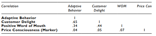
Let’s initially examine the correlation of Adaptive Behavior and Customer Delight. The unadjusted correlation is .65.The second lowest correlation of Price Consciousness (marker) to any other construct in the model is .05. Next, let’s get the adjusted correlation for Adaptive Behavior and Customer Delight.

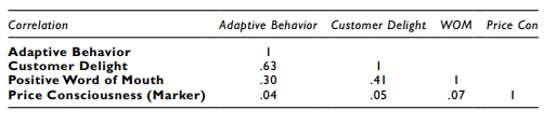
The adjusted correlation is .63. Since we are parceling out a level of correlation, your adjusted correlation should be smaller.You will need to find the adjusted correlation for each value in the correlation analysis for the constructs of your model.

Here is the adjusted correlation for each construct with the marker variable’s influence removed from the other constructs.

Once you get the adjusted correlation for every construct of your study, you will then use this adjusted correlation matrix as your input for your AMOS model.To see how to use a cor- relation matrix as the input of your model, see Chapter 5.

The downside of using this technique is you are asking an “out of the blue” question in your survey, which could confuse the respondent. The biggest concern is this technique almost necessitates that you use composite variables in your analysis. One of the primary strengths of SEM is to model measurement error. With this technique of using an adjusted correlation matrix as your input, you are just examining the relationships between composite variables, which could present a slightly different picture of your results compared to a model that had all the indicators for each construct included in the analysis.

3. Include a Latent Common Method Factor—the most popular way to handle common method bias is to include a common method factor in your A common method factor is a latent variable that has a direct relationship with each construct’s indicators. The com- mon method factor will represent and account for variance across constructs (due to the potential methods bias). You will first model your CFA, then you will include a latent variable in the model with no indicators. Label this variable “Common_Method” or whatever you want in order to remember that this is the common method construct. From this common method construct, you will start drawing relationships from the con- struct to all the indicators in the model.You will include a direct relationship from the unobserved common method latent construct to every indicator in the model.You might want to go about this in a systematic manner so that you do not miss a relationship to an indicator. With a CFA that has a large number of constructs, this can be a substantial number of relationships, so my best advice is to start adding relationships one construct at a time until all the indicators have a relationship to the unobservable common method factor.

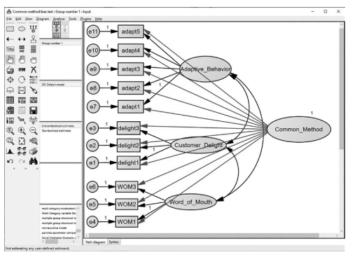
Figure 4.36 Example of Common Method Factor With a Relationship to Every Indicator

After drawing a path from the common method construct to all the indicators, you will need to constrain all the relationships from the common method factor to be equal. We are doing this to see what is the common influence across all the indicators. If common method bias is present, it should affect all the variables of the survey equally. Right click on one of the relationships (arrows) from the common method construct; the Object Properties window should appear. Under the Parameters tab at the top, put a letter in the “regression weight” line. In this example, I labeled the regression weight simply “a”, but you could call it anything you want. After labeling the parameter, you can cancel out of this screen.

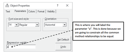
Figure 4.37 Constraining All Relationships to “a” in Common Method Bias Test

You can go into each relationship and constrain all the parameters to the letter “a”, but this might be extremely time consuming if you have a large number of indicators. AMOS has a function that lets you copy a constraint to other relationships. So, we will copy this constraint of letter “a” and paste it in all other relationships from the common method construct. To do this, the first thing you need to do is select all the other relationships from the common method variable (do not select the one that is already constrained with an “a”). The easiest way to do this is to use the (select) button and select each relationship.You can also hold down the left-click button on your mouse and drag over the relationships, and it will also highlight them.

Next, you need to select the “Drag Properties” button . A pop-up window will appear. Select “Parameter Constraints” in the Drag Properties window. Now, go back to the relation- ship that has the regression weight labeled “a” and drag the “a” to all the other highlighted relationships. Make sure the “Drag Properties” pop-up window is active on the screen, or it will not perform the drag function.The Drag Properties icon is a handy function, especially if you have a larger number of indicators.

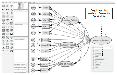
Figure 4.38 Using the Drag Function to Constrain All the Relationships to “a”

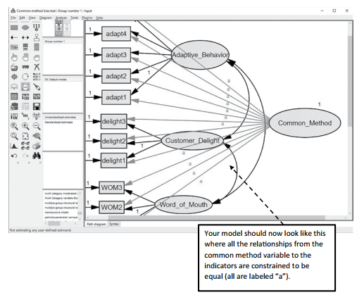
Figure 4.39 Example of All Relationships Constrained in Common Method Test

Before moving forward, it is a good idea to hit the “Deselect All Objects” icon  so that you are not having any unintended action with the high- lighted relationships from the com- mon method factor. After constraining all the relationships to be equal, you next need to right click in the unob- servable common method variable. The Object Properties window will appear. You should set the variance of the unobserved construct to “1”. This is done because we are concerned only about the impact of the potential bias to the indicators of our model.

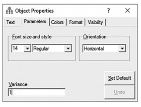
Figure 4.40 Setting the Variance to “1” in Unob- servable Common Method Variable

Next, you will run the analysis for the model . AMOS will initially warn you that your unobserved variables in the CFA do not have a covariance to the common_method construct.

You do not need to covary your constructs in the model with the common_method construct. Just hit the “Proceed with the Analysis” button to continue without adding additional covari- ances.After the analysis finishes, go into the output and go to the model fit link.With the com- mon method test, we will perform a chi-square difference test to determine if bias is present. Specifically, you are concerned with the chi-square values of the CFA model. The CFA com- parison will examine what the chi-square value was for your CFA when the common method construct was not included, and then a comparison will be made to the chi-square value of the CFA when the common method construct was included. In the analysis, you should see only 1 degree of freedom difference between the two models. Remember, we constrained all the relationships in the common method construct model to be equal. Hence, we need to see if the difference in chi-square is significant which would indicate a common method bias.

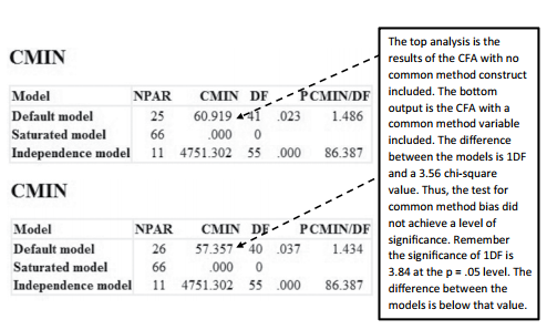
Figure 4.41 Difference of Chi-Square for Common Method Test

Source: Thakkar, J.J. (2020). “Procedural Steps in Structural Equation Modelling”. In: Structural Equation Modelling. Studies in Systems, Decision and Control, vol 285. Springer, Singapore.