Evaluating Heterogeneity among Effect Sizes

In Figure 8.1, all of the studies had confidence intervals that contained the vertical line representing the overall population effect size. This situation is called homogeneity—most of the studies capture a common population effect size, and the differences that do exist among their point estimates of effect sizes (i.e., the circles in Figure 8.1) are no more than expected by random­sampling fluctuations. Although not every study’s confidence interval needs to overlap with a common effect size in order to conclude homogeneity (these are, after all, only probabilistic confidence intervals), most should. More for­mally, there is an expectable amount of deviation among study effect size estimates, based on their standard errors of estimate, and you can compare whether the actual observed deviation among your study effect sizes exceeds this expected value.

If the deviation among studies does exceed the amount of expectable deviation, you conclude (with some qualifications I describe below) that the effect sizes are heterogeneous. In other words, the single vertical line in Fig­ure 8.1 representing a single common effect size is not adequate. In the situa­tion of heterogeneous effect sizes, you have three options: (1) ignore the het­erogeneity and analyze the data as if it is homogeneous (as you might expect, the least justifiable choice); (2) conduct moderator analyses (see Chapter 9), which attempt to predict between-study differences in effect size using the characteristics of studies coded (e.g., methodological features, characteristics of the sample); or (3) fit an alternative model to that of Figure 8.1, in which the population effect size is modeled as a distribution rather than a vertical line (a random-effects model; see Chapter 10).

1. Significance Test of Heterogeneity

The heterogeneity (vs. homogeneity) of effect sizes is frequently evaluated by calculating a statistic Q. This test is called either a homogeneity test or, less commonly, a heterogeneity test; other terms used include simply a Q test or Hedges’s test for homogeneity (or Hedges’s Q test). I prefer the term “heteroge­neity test” given that the alternate hypothesis is of heterogeneity, and therefore a statistically significant result implies heterogeneity. This test involves com­puting a value (Q) that represents the amount of heterogeneity in effect sizes among studies in your meta-analysis using the following equation (Cochran, 1954; Hedges & Olkin, 1985, p. 123; Lipsey & Wilson, 2001, p. 116):

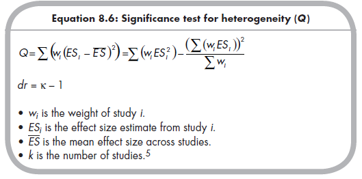
The left portion of this equation is the definitional formula for Q and is relatively straightforward to understand. One portion of this equation simply computes the (squared) deviation between the effect size from each study and the mean effect size across studies, which is your best estimate of the population effect size, or vertical line of Figure 8.1. This squared deviation is multiplied by the study weight, which you recall (Equation 8.1) is the inverse of the squared standard error of that study. In other words, the equation is essentially the ratio of the (squared) deviations between the effect sizes to the (squared) expected deviation. Therefore, when studies are homogeneous, you expect this ratio to be close to 1.0 for each study, and so the sum of this ratio across all studies is going to be approximately equal to the number of studies (k) minus 1 (the minus 1 is due to the fact that the population effect size is estimated by your mean effect size from your sample of studies). When stud­ies are heterogeneous, you expect the (squared) deviations between studies and mean effect sizes to be larger than the (squared) expected deviations, or standard errors. Therefore, the ratio will be greater than 1.0 for most stud­ies, and the resulting sum of this ratio across studies will be higher than the number of studies minus 1.

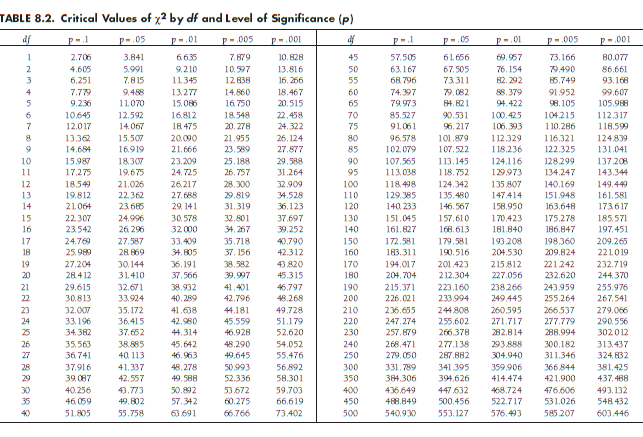
Exactly how high should Q be before you conclude heterogeneity? Under the null hypothesis of homogeneity, the Q statistic is distributed as C² with df = k – 1. Therefore, you can look up the value of the Q with a particular df in any chi-square table, such as that of Table 8.2,⁶ to determine whether the effect sizes are more heterogeneous than expected by sampling variability alone.

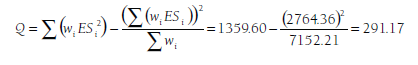
The equation in the right portion of Equation 8.5 provides the same value of Q as the definitional formula on the left (it is simply an algebraic rearrangement). However, this computational equation is easier to compute from your meta-analytic database. Specifically, you need three variables (or columns in a spreadsheet): the Wj and WjESj that you already calculated to compute the mean effect size, and WjESi² that can be easily calculated. To illustrate, the rightmost column of Table 8.1 displays this WjESi² for each of the 22 studies in the running example, with the sum (ZWjESj²) found to be 1359.60 (bottom of table). Given the previously computed (when calculating the mean effect size) sums, Swj = 7152.21 and SwjESi = 2764.36, you can com­pute the heterogeneity statistic in this example using Equation 8.6,

You can evaluate this Q value using df = k – 1 = 22 – 1 = 21. From Table 8.2, you see that this value is statistically significant (p < .001). As I describe in the next section, this statistically significant Q leads us to reject the null hypothesis of homogeneity and conclude the alternate hypothesis of hetero­geneity.

2. Interpreting the Test of Heterogeneity

The Q statistic is used to evaluate the null hypothesis of homogeneity ver­sus the alternate hypothesis of heterogeneity. If the Q exceeds the critical C² value given the df and level of statistical significance chosen (see Table 8.2), then you conclude that the effect sizes are heterogeneous. That is, you would conclude that the effect sizes are not all estimates of a single popula-tion value, but rather, multiple population values. If Q does not exceed this value, then you fail to reject the null hypothesis of homogeneity.

This description makes clear that evaluation of Q (i.e., of heterogeneity vs. homogeneity) is a statistical hypothesis test. This observation implies two cautions in interpreting findings regarding Q. First, you need to be aware that this test of heterogeneity provides us information about the likelihood of results being homogeneous versus heterogeneous, but does not tell us the magnitude of heterogeneity if it exists (a consideration you should be par­ticularly sensitive to, given your attention to effect sizes as a meta-analyst). I describe an alternative way to quantify the magnitude of heterogeneity in the next Section (8.4.3). Second, you need to consider the statistical power of this heterogeneity test—if you have inadequate power, then you should be very cautious in interpreting a nonsignificant result as evidence of homogeneity (the null hypothesis). I describe the statistical power of this test in Section

3. An Alternative Representation of Heterogeneity

Whereas the Q statistic and associated significance test for heterogeneity can be useful in drawing conclusions about whether a set of effect sizes in your meta-analysis are heterogeneous versus homogeneous, they do not indicate how heterogeneous the effect sizes are (with heterogeneity of zero represent­ing homogeneity). One useful index of heterogeneity in your meta-analysis is the I² index. This index is interpreted as the percentage of variability among effect sizes that exists between studies relative to the total variability among effect sizes (Higgins & Thompson, 2002; Huedo-Medina, Sanchez-Meca, Marin-Martinez, & Botella, 2006). The I² index is computed using the fol­lowing equation (Higgins & Thompson, 2002; Huedo-Medina et al., 2006):

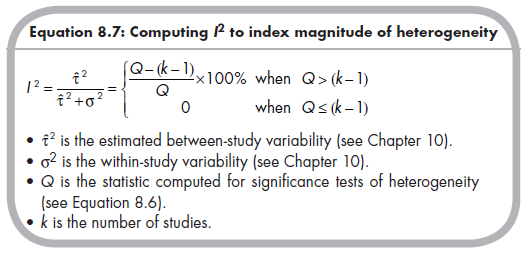
The left portion of this equation uses terms that I will not describe until Chapter 10, so I defer discussion of this portion for now. The right portion of the equation uses the previously computed test statistic for heterogeneity (Q) and the number of studies in the meta-analysis (k). The right portion of the equation actually contains a logical statement, whereby I² is bounded at zero when Q is less than expected under the null hypothesis of homogeneity (lower possibility), but the more common situation is the upper possibil­ity. Here, the denominator consists of Q, which can roughly be considered the total heterogeneity among effect sizes, whereas the numerator consists of what can roughly be considered the total heterogeneity minus the expected heterogeneity given only sampling fluctuations. In other words, the ratio is roughly the between-study variability (total minus within-study sampling variability) relative to total variability, put onto a percentage (i.e., 0 to 100%) scale.

I² is therefore a readily interpretable index of the magnitude of hetero­geneity among studies in your meta-analysis, and it is also useful in com­paring heterogeneity across different meta-analyses. Unfortunately, because it is rather new, it has not been frequently used in meta-analyses, and it is therefore difficult to offer suggestions about what constitutes small, medium, or large amounts of heterogeneity.⁷ In the absence of better guidelines, I offer the following suggestions of Huedo-Medina and colleagues (2006) that I² = 25% is a small amount of heterogeneity, I² ~ 50% is a medium amount of heterogeneity, and I² ~ 75% is a large amount of heterogeneity (as mentioned, I² ~ 0% represents homogeneity). In the example meta-analysis of relational aggression with peer rejection I described earlier, I² = 92.8%.

4. Statistical Power in Testing Heterogeneity

Although the Q test of heterogeneity is a statistical significance test, many meta-analysts make conclusions of homogeneity when they fail to reject the null hypothesis. This practice is counter to the well-known caution in pri­mary data analysis that you cannot accept the null hypothesis (rather, you simply fail to reject it). On the other hand, if there is adequate statistical power to detect heterogeneity and the results of the Q statistic are not sig­nificant, then perhaps conclusions of homogeneity—or at least the absence of substantial heterogeneity—can be reasonably made. The extent to which this argument is tenable depends on the statistical power of your heterogene­ity test.

Computing the statistical power of a heterogeneity test is extremely complex, as it is determined by the number of studies, the standard errors of effect size estimates for these studies (which is largely determined by sample size), the magnitude of heterogeneity, the theoretical distribution of effect sizes around a population mean (e.g., the extent to which an effect size index is normally [e.g., Z is approximately normally distributed] vs. non-normally [e.g., r is skewed, especially at values far from zero] distributed), and the extent to which assumptions of the effect size estimates from each study are violated (e.g., assuming equal variance between two groups when this is not true) (see, e.g., Alexander, Scozzaro, & Borodkin, 1989; Harwell, 1997). In this regard, computing the statistical power of the heterogeneity test for your particular meta-analysis is very difficult, and likely precisely possible only with complex computer simulations.

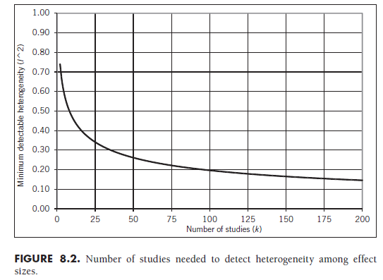
Given this complexity, I propose a less precise but much simpler approach to evaluating whether your meta-analysis has adequate statistical power to detect heterogeneity. First, you should determine a value of I² (see previous subsection) that represents the minimum magnitude of heterogeneity that you believe is important (or, conversely, the maximum amount of heterogene­ity that you consider inconsequential enough to ignore). Then, consult Figure 8.2 to determine whether the number of studies in your meta-analysis can conclude that your specified amount of heterogeneity (I²) will be detected. This figure displays the minimum level of I² that will result in a statistically significant value of Q for a given number of studies, based on p = .05. If the figure indicates that the number of studies in your meta-analysis could detect a smaller level of I² than what you specified, it is reasonable to conclude that the test of heterogeneity in your meta-analysis is adequate. I stress that this is only a rough guide, which I offer only as a simpler alternative to more com­plex power analyses; however, I feel that it is likely adequate for most meta­analyses.⁸ Accepting Figure 8.2 as a rough method of determining whether tests of heterogeneity have adequate statistical power, it becomes clear that this test is generally quite powerful. Based on the suggestions of I² ~ 25%, 50%, and 75% representing small, medium, and large amounts of heteroge­neity, respectively, you see that meta-analyses consisting of 56 studies can detect small heterogeneity, those with as few as 9 studies can detect medium heterogeneity, and all meta-analyses (i.e., combination of two or more stud­ies) can detect large heterogeneity.

Before concluding that the test of heterogeneity is typically high in sta­tistical power, you should consider that the I² index is the percentage ratio of between-study variance to total variance, with total variance made up of both between- and within-study variance. Given the same dispersion of effect sizes from a collection of studies with large standard errors (small samples) rather than small standard errors (large samples), the within-study variance will be larger and the I² will therefore be smaller (because this larger within- study variance goes into the numerator or Equation 8.7). Given these situ­ations of large standard errors (small sample sizes) among studies, the test of heterogeneity can actually have low power because the I² is smaller than expected (see Harwell, 1997, for a demonstration of situations in which the test has low statistical power). For this reason, it is important to carefully consider what values of I² are meaningful given the situation of your own meta-analysis and those in similar situations, more so than relying too heav­ily on guidelines such as those I have provided.

Source: Card Noel A. (2015), Applied Meta-Analysis for Social Science Research, The Guilford Press; Annotated edition.