Continuous Moderators in meta-analysis

Continuous moderators in meta-analysis are coded study variables that can be considered to vary along a continuum of possible values. For example, mean characteristics of the sample (age, SES, percentage of ethnic minorities, percentage male or percentage female) or methodology (e.g., dose of a drug, number of therapy sessions in intervention) might be evaluated as continu­ous moderators. Just as the evaluation of categorical moderators relied on an adaptation of ANOVA, the evaluation of continuous moderators relies on an adaptation of regression. Specifically, test of continuous moderation involves (weighted) regression of the effect sizes (dependent variable) onto the con­tinuous moderator (independent variable, or predictor). Significant predic­tion indicates that the effect sizes vary in a linear manner with the continu­ous moderator; in other words, this moderator systematically relates to the association between X and Y.

The adaptation of standard regression of effect sizes onto a continuous predictor that is key to meta-analytic moderator analysis is the “weighted” I parenthetically stated. Here, the regression analysis is weighted by the inverse variance weight, w (see Chapter 8). This weighting has three implications. First, as is desirable (see Chapter 8), studies with more precise effect size esti­mates will be given more weight in the analysis than those with less precise estimates. Second, the mean squares of the regression (standard output, often in an ANOVA table, of all standard statistical packages such as SPSS or SAS) represents the heterogeneity among the effect sizes that is accounted for by the linear prediction of the continuous moderator. You use this value to eval­uate the statistical significance of the regression model. Third, this weight­ing impacts the standard errors of the regression coefficients. Although the regression coefficients themselves are accurate and directly interpretable (e.g., are effect sizes larger or smaller when values of the moderator are greater?), the standard errors of the regression coefficients are not correct and need to be hand calculated (which, fortunately, is simple).

Because this weighted regression approach to testing continuous moder­ators is most clearly illustrated through example, let me return to the sample meta-analysis of associations between relational aggression and peer rejec­tion. As shown in Table 9.2, I coded the mean age (in years) of the samples for these 22 studies, and I want to evaluate whether age moderates the asso-ciations between relational aggression and rejection. To do so, I regress the effect sizes (Fisher’s transformation of the correlation between relational aggression and rejection, Z_r) onto the hypothesized continuous moderator age, using the familiar regression equation. Z_r = Bq + B]_(Age) + e, with w as a weight. To do this, I use a standard statistical software package such as SPSS or SAS. In SPSS, I would specify Z_r as the dependent variable, age as the inde­pendent variable, and w as the WLS (weighted least squares) weight.

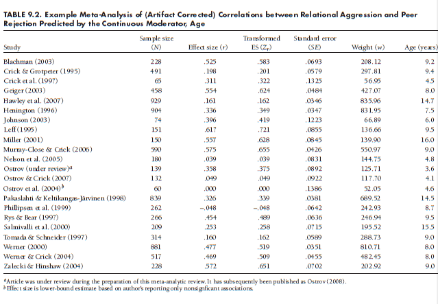
The results give six pieces of information of interest: from an ANOVA table, (1) the sum of square of the regression model (SSregression or SSmodel) = 9.312; (2) the residual sum of squares3 (SSresidual or SSerror) = 281.983; and (3) the residual mean squares (MSresidual or MSerror) = 14.099; and from a table of coefficients, (4) the unstandardized regression coefficient (B1) = –.0112 with (5) an associated standard error = .0138; and (6) the intercept (B0) = .496. The SSregression is the heterogeneity accounted for by the linear regression model; it is often reported in published meta-analysesas Qr egression and is evaluated for statistical significance by comparing the value to a c2 distribution (Table 8.2 or using calculators such as Excel’s “chiinv” function) with df = number of predictors (here, df = 1). In this example, the value of 9.312 is considered statistically significant by standard criteria (p = .0023), so I conclude that there is moderation of the association between relational
aggression and rejection by age.

Because this analysis included only one predictor, the statistical signifi­cance of the model informs the statistical significance of the single predictor. However, when including multiple predictors (see next section), it is useful to also evaluate statistical significance by examining the regression coefficients and their standard errors. In this example, the unstandardized regression coefficient was -.0112, and its standard error, as computed by the statistical analysis program, was .0138. However, this standard error is inaccurate, and must be adjusted. This adjustment is to divide the standard error from the output by the square root of the residual mean square:

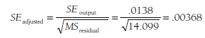
I then evaluate the statistical significance of this predictor by dividing the regression coefficient (B1) by this adjusted standard error, Z = -.0112/.00368 = -3.05, considering this Z value according to the standard normal deviate (i.e., Z) distribution to yield a two-tailed p (here, p = .0023). Note that in this example with a single predictor, the statistical significance of the regression model and of the single regression coefficient are identical, given that Z² = x²(df=1) (i.e., -3.05² = 9.31).

To interpret this moderation, it is useful to compute implied effect sizes at different levels of the continuous moderator. Given the intercept (Bq = .096) and regression coefficient of age (B]_ = -.0112), I can compute the pre­dicted effect sizes at various ages using the equation Z_r = Bq + Bi (Age) = .496 – .0112 (Age). For illustration of this moderation, I would choose rep­resentative values of the moderator (age) that fall within the range observed among these studies and make some conceptual sense; in this example, I might choose the ages of 5, 10, and 15 years. I then successively insert these values for age into the prediction equation, yielding implied Z_rs = .440, .384, and .328, respectively. I then back-transform these implied Z_rs (or any other transformed effect sizes) into their meaningful metric for reporting: implied rs = .41, .37, and .32, respectively.

Source: Card Noel A. (2015), Applied Meta-Analysis for Social Science Research, The Guilford Press; Annotated edition.