There are relatively few instances of meta-analyzing single variables, yet this information could be potentially valuable. At least three types of information regarding single variables could be important: (1) the mean level of individuals on a continuous variable; (2) the proportions of individuals falling into a particular category of a categorical variable; and (3) the amount of variability (or standard deviation), in a continuous variable.
1. Mean Level on Variable
Meta-analysis of reported means on a single variable may have great value. One potential is that meta-analytic combination (see Chapters 8 and 9) allows you to obtain a more precise estimate of this mean than might be obtained in primary studies, especially when those primary studies have small sample sizes. Perhaps more importantly, meta-analytic comparison (see Chapter 10) allows you to identify potential reasons why means differ across studies (e.g., methodological differences such as condition or reporter; sample characteristics such as age or ethnicity). Thus, the meta-analysis of means of single variables has considerable value.
At the same time, there is also an important limiting consideration in the meta-analysis of means in that the primary studies must typically report this value in the same metric. For example, if one study measures the variable of interest on a 0-4 scale, whereas another uses a 1-100 scale, it usually does not make sense to combine or compare means across these studies.1 Some exceptions can be considered, however. The first exception is if the different scales are due to the primary study authors scoring comparable measures in different ways, then it is usually possible to transform one of the scales to the metric of the other. For example, if two primary studies both use a 6-item scale with items having values from 1 to 5, one study may form a composite by averaging the items, whereas the other forms a composite by summing the items. In this case, it would be possible to transform one of the two means to the same scale of the other (i.e., multiplying the average by 6 to obtain the sum, or dividing the sum by 6 to obtain the average), and the means of the two studies could then be combined and compared. A second, more general exception is that it might usually be possible to transform studies using different scales into a common metric. From the example I provided of one study using a 0-4 scale and the other using a 1-100 scale, it is possible to transform a mean on one scale to an equivalent mean on the other using the following equation:
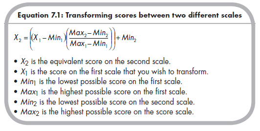
A caution in using different scales is that even if both studies use a common range of scores (e.g., 0-4), it is probably only meaningful to combine and compare means if the studies used the same anchor points (e.g., if one used response options of never, rarely, sometimes, often, and always, whereas the other used 0 times, once, 2-3 times, 4-6 times, and 7 or more times, it would make little sense to combine or compare these studies). This may prove an especially difficult obstacle if you are attempting to combine multiple scales in which scores from one scale are transformed to scores of another using Equation 7.1. This requirement of primary studies reporting the variable on the same—or at least a comparable—metric means that you will often include only studies using the same measure (e.g., a particular measure of depression, such as the Children’s Depression Inventory; Kovacs, 1992) or else very similar measures (e.g., child- and teacher-reported aggression using parallel items and response options). I suspect that this rather restrictive requirement is the primary reason why meta-analysis of means is not more common. If you are using different but similar measures, or transformations to place values of different measures on a common scale, I highly recommend evaluating the measure as a moderator (see Chapter 9).
If you do have a situation in which the combination or comparison of means is feasible, computing this effect size (and its standard error) is straightforward. The equation for computing a mean is well known, but I reproduce it here:
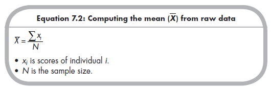
However, it is typically not necessary (or possible) for you to compute this mean, as this is usually reported within the primary study. Therefore, coding the mean, which is an effect size (of the central tendency of a single variable), is usually straightforward.
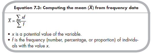
Occasionally, however, the primary studies will report frequency tables rather than means for variables with a small number of potential options. For example, a primary study might report the number or proportion of individuals scoring 0, the number or proportion scoring 1, and so on, on a measure that has possible options of 0, 1, 2, 3, and 4. Here, you can use these frequencies of different scores to re-create the raw data and then compute the mean from these data (using Equation 7.2). An easier way to compute this mean is using the following equivalent formula provided by Lipsey and Wilson (2001, p. 176), summing over all potential values of a variable:
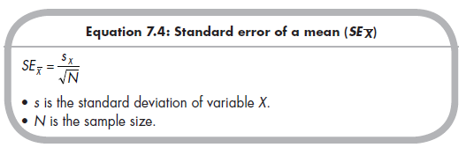
Before ending my discussion of calculating the mean as an effect size, it is important to consider the standard error of this estimate of the mean (which is used for weighting in the meta-analysis; see Chapter 8). To compute the standard error of a study’s estimate of the mean, you must obtain the (population estimate of the) standard deviation (s) and sample size (N) from that study, which are then used in the following equation:
After computing the mean and standard error of the mean for each study, you can then meta-analytically combine and compare results across studies using techniques described later in this book (see Chapters 8-10).
2. Proportion of Individuals in categories
Whereas the mean is a useful effect size for the typical score (i.e., central tendency) of a single continuous variable, the proportion is a useful effect size for a particular category of a categorical variable. For example, we may be interested in the proportion of children who are aggressive or the proportion of individuals who meet certain criteria for rejected social status, if we believe the meaningful conceptualization of aggression or rejection is categorical. In these cases, we are interested in the prevalence of an affirmative instance of a single dichotomous variable.2
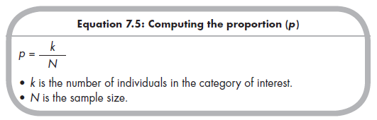
This proportion is often either directly reported in primary studies (as either a proportion or percentage, which can be divided by 100 to obtain the proportion), or else can be computed from the reported frequency falling in this category (k) relative to the total sample size (N):
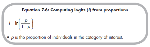
This proportion works well as an effect size in many situations, but is problematic when proportions are far from 0.50.3 For this reason, it is useful to transform proportions (p) into logits (l) prior to meta-analytic combination or comparison:
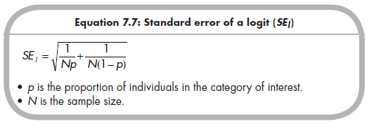
This logit has the following standard error dependent on the proportion (p) and sample size (N) (Lipsey & Wilson, 2001, p. 40):
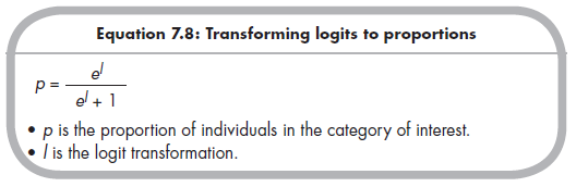
Analyses would then be performed on the logit (l), weighted by the standard error (SEj) as described in Chapters 8 through 10. For reporting, it is useful to back-transform results (e.g., mean effect size) in logits (l) back to proportions (p), using the following equation:
3. Variances and Standard Deviations
Few meta-analyses have used variances, or the equivalent standard deviation (the square root of the variance), as effect sizes. However, the magnitude of interindividual difference is a potentially interesting focus, so I offer this brief description of using these as effect sizes for meta-analysis.
The standard deviation, which is the square root of the variance, is calculated from raw data as follows:
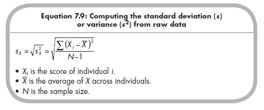
This equation is the unbiased estimate of population standard deviation (and the square root of variance) from a sample (versus a description of the sample variability, which would be computed using N rather than N – 1 in the denominator). This is also the statistic commonly reported in primary research. In fact, you will almost never need to calculate this standard deviation, as doing so requires raw data that are typically not available. Fortu-nately, standard deviations (or variances) are nearly always reported as basic descriptive information in primary studies.4
To meta-analytically combine or compare standard deviations (or variances) across studies, you must also compute the standard error used for weighting (see Chapter 8). The standard error of the standard deviation is a function of the standard deviation itself and the sample size (Pigott & Wu, 2008):
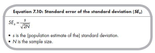
The standard error of a variance estimate, as you might expect, is simply Equation 7.10 squared (i.e., SEs2 = s 2/2N)
At this point, you may have concluded that meta-analysis of standard deviations (and therefore variances) is straightforward. To a large extent this is true, though three qualifiers should be noted. First, as with the mean, it is necessary that the studies included all use the same measure, or at least measures that can be placed on the same scale. Just as it would make little sense to combine means from studies’ incomparable scales, it does not make sense to combine magnitudes of individual difference (i.e., standard deviations) from incomparable scales. Second, standard deviations are not exactly normally distributed, especially with small samples. Following the suggestion of Pigott and Wu (2008), I suggest that you do not attempt to meta-analyze standard deviations if many studies have sample sizes less than 25. A third consideration involves the possibility of diminished standard deviations due to ceiling or floor effects. Ceiling effects occur when most individuals in a study score near the top of the scale, and floor effects occur when most individuals score near the bottom of the scale. In both situations, estimates of standard deviation are lowered because there is less “room” for individuals to vary given the constraints of the scale. For example, if we administered a third- grade math test to graduate students, we would expect that most of them would score near the maximum of the test, and the real individual variability in math skills would not be captured by the observed variability in scores on this test. I suggest two strategies for avoiding this potential biasing effect: (1) visually observe the means of studies and consider excluding those studies where the mean is close to the bottom or top of the scale, and (2) compute a correlation across studies between means and standard deviations—the presence of an association suggests a potential floor or ceiling effect, whereas the absence of association would suggest this bias is not present.5
Source: Card Noel A. (2015), Applied Meta-Analysis for Social Science Research, The Guilford Press; Annotated edition.
25 Aug 2021
25 Aug 2021
25 Aug 2021
25 Aug 2021
25 Aug 2021
24 Aug 2021