A General Multiple Regression Framework for Moderation in meta-analysis

After considering the regression approach to analyzing continuous modera­tors (previous section), you are probably wondering whether this approach allows for evaluation of multiple moderators—it does. However, before con­sidering inclusion of multiple moderators, I think it is useful to take a step back to consider how a regression approach can serve as a general approach to evaluating moderators in meta-analysis (in this context, the analyses are sometimes referred to as meta-regression). In this section, I describe how an empty (intercept-only) model accomplishes basic tests of mean effect size and heterogeneity (9.3.1), how you can evaluate categorical moderators in this framework through the use of dummy codes (9.3.2), and how this flexible approach can be used to consider unique moderation of a wide range of coded study characteristics (9.3.3). I will then draw general conclusions about this framework and suggest some more complex possibilities. I write this section with the assumption that you have a solid grounding in multiple regression; if not, you can read this section trying to obtain the “gist” of the ideas (for a thorough instruction of multiple regression, see Cohen et al., 2003).

1. The Empty Model for Computing Average Effect Size and Heterogeneity

An empty model in regression is one in which the dependent variable is regressed against no predictors, but only a constant (i.e., the value of 1 for all cases). This is represented in the following equation, which includes only an intercept (constant) as a predictor:

Performing a weighted regression of effect sizes predicted only by a constant will yield information about the weighted mean effect size and the heterogeneity, and therefore might serve as a useful initial analysis that is less tedious than the hand-spreadsheet-calculations I described in Chapter 8. Considering the example of 22 studies of relational aggression and peer rejection summarized in Table 9.2, I perform the following steps: First, I place the effect sizes (Z_rs) and inverse variance weights (w) into a statistical software package (e.g., SPSS or SAS). I then create a variable in which every study had the value 1 (the constant). Finally, I regress effect sizes onto this constant, weighted by w, specifying no intercept (i.e., having the program not automatically include the constant in the model, as I am using the con­stant as a predictor). The unstandardized regression coefficient is .387, which represents the mean effect size (as Z_r). The standard error of this regression coefficient from the program is adjusted as described above,

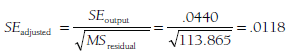
to yield the standard error of this mean effect size for use in significance test­ing or estimating confidence intervals. Finally, the residual sum of squares (55_resjdual or SS_error) = 291.17 is the heterogeneity (Q) statistic, evaluated as C² with 21 (number studies – 1) degrees of freedom. These results are identi­cal to those reported in Chapter 8 and illustrate how the empty model can be used to compute the mean effect size, make inferences about this mean, and evaluate the heterogeneity of effect sizes across studies.

2. Evaluating categorical Moderators

In primary data analysis, it has long been recognized that ANOVA is sim­ply a special case of multiple regression (e.g., Cohen, 1968). The same com­ parability applies to meta-analytic evaluation of categorical moderators. As with translation of ANOVA into multiple regression in primary analysis, the “trick” is to create a series of dichotomous variables that fully capture the different groups. The most common approach is through the use of dummy variables.

To illustrate the use of dummy variables in analyzing continuous mod­erators, consider the data from Table 9.3, which consists of 27 effect sizes (from 22 studies, as in Table 9.2) using four methods of measuring rela­tional aggression (previously summarized in Table 9.1). As with the ANOVA approach, I want to evaluate whether the method of assessing aggression moderates the associations between relational aggression and rejection. To perform this same evaluation in a regression framework, I need to compute three dummy codes (number of groups minus 1) to represent group member­ship. If I selected observational methods as my reference group, then I would assign the value 0 for all three dummy codes for studies using observational methods. I could make the first dummy code represent parent report (vs. observation) and assign values of 1 to this variable for all studies using this method and values of 0 for all studies that do not. Similarly, I could make dummy variable 2 represent peer report and dummy variable 3 represent teacher report. These dummy codes are displayed in Table 9.3 as DV1, DV2, and DV3 (for now, ignore the column labeled “Age” and everything to the right of it; I will use these data below).

To evaluate moderation by reporter within a multiple regression frame­work, I regress effect sizes onto the dummy variables representing group membership (in this case, three dummy variables), weighted by the inverse variance weight, w. This is expressed in the following equation:

Using a statistical software package (e.g., SPSS or SAS), I regress the effect sizes (Z_rs) onto the three dummy variables (DV1, DV2, and DV3), weighted by the inverse variance weight (w) (here, I am requesting that the program include the constant in the model because I have not used the constant as a predictor). The output from the ANOVA table of this regression parallels the results from the ANOVA I described in Section 9.1: The total sum of squares (SS_total) provides the total heterogeneity (Qtotal) = 350.71; the residual or error sum of squares (SS_resjd_ual or SS_error) provides the within-group heterogeneity (Q_within) = 285.57; and the regression or model sum of squares (SS_reqression or SS_model) provides the between-group heterogeneity (Qb_etween) = 65.14. This last value is compared to a c² distribution (e.g., Table 8.2) to evaluate whether the categorical moderator is significant. This regression analysis also yields coefficients and their (incorrect) standard errors. If I adjust these standard errors, I can evaluate the statistical significance of the regression coefficients as indicative of whether each group differs from the reference group. To illus­trate: In this example, in which I coded observational methods as the refer­ence group, I could consider the regression coefficient of DV2 (denoting use of peer reports) = .301 by dividing it by the corrected standard error

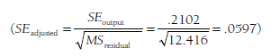
to yield Z = .301 / .0597 = 5.05. I would thus conclude that studies using peer-report methods yield larger effect sizes than studies using observational methods. More generally, I could compute the implied values of each of the four methods via the prediction equation comprised of the intercept and regression coefficients for the dummy variables:

Because I used observational methods as my reference group, the implied mean effect size for this group is Z_r = .097. For studies using parent reports (the first dummy variable), the implied effect size is Z_r = .583 (.097 + .486); for studies using peer reports (the second dummy variable), the implied effect size is Z_r = .398 (.097 + .301); and so on. When using transformed effect sizes such as Z_r, you should transform these implied values back to the more intui­tive metric (e.g., r) for reporting.

As in primary analysis (see Cohen & Cohen, 1983), dummy variables represent just one of several options for coding group membership in meta­analytic tests of categorical moderators. Dummy variables have the advan-tages of explicitly comparing all groups to a reference group, which might be of central interest in some analyses. However, dummy variables have the dis­advantages of not allowing for easy comparisons between groups that are not the reference group (e.g., between peer and teacher reports in the example just presented) and that are not centered around 0 (a consideration I describe below). Effects coding (see Cohen & Cohen, 1983, p. 198) still relies on a ref­erence group, but centers on the independent variables. For example, effects for four groups would use three effects codes, which might be —A, —A, and —A for the reference group; A, 0, and 0 for the second group; 0, A, and 0 for the third group; and 0, 0, and A for the fourth group.⁴ Another alternative is contrast coding (Cohen & Cohen, 1983, p. 204), which allows for flexibility in creating specific planned comparisons among subsets of groups.

3. Evaluating Multiple Moderators

Having considered the regression framework for analyzing mean effect sizes, categorical moderators, and a single continuous moderator, you have likely inferred that this multiple regression approach can be used to evaluate multi­ple moderators. Doing so is no more complex than entering multiple categori­cal (represented with one or more dummy variables, effects codes, or contrast codes) or continuous predictors in this meta-analytic multiple regression.

However, one important consideration is that of centering (i.e., subtract­ing the mean value of a predictor from the values of this predictor). Although the statistical significance of either the overall model or individual predictors will not be influenced by whether or not you center, centering does offer two advantages. First, it permits more intuitive interpretation of the intercept as the mean effect size across studies. Second, it removes nonessential colinear­ity when evaluating interaction or power polynomial terms. To appropriately center predictors for this type of regression, you perform two steps. First, you compute the weighted (by inverse variance weights, w) average value of each predictor. Second, you compute a centered predictor variable by subtracting this weighted mean from scores on the original (uncentered) variable for each study. This process works for either continuous variables or dichoto­mous variables (this method of centering dummy variables converts them to effects codes).

To illustrate centering and evaluation of multiple moderators, I turn again to the example meta-analysis of the associations between relational aggression and rejection. In this illustration, I want to evaluate moderation both by method of measuring aggression and by age. Specifically, I want to evaluate whether either uniquely moderates these effect sizes (controlling for any overlap between method and age that may exist among these studies; see Section 9.4). Table 9.3 displays these 27 effect sizes (from 22 studies), as well as values for the two predictors: three dummy variables denoting the four categorical levels of method, and the continuous variable age. To create the centered variables, I first computed the weighted mean for each of the three dummy variables and age; these values were .0265, .8206, .1155, and 9.533, respectively.⁵ I then subtracted these values from scores on each of these four variables, resulting in the four centered variables shown on the right side of Table 9.3. I have labeled the three centered dummy codes as effects codes (EC1, EC2, and EC3), and the centered age variable “C_Age.”

When I then regress the effect size (Z_r) onto these four predictors (EC1, EC2, EC3, and C_Age), weighted by w, I obtain SS_reg_ressi_on = 93.46. Evaluat­ing this amount of heterogeneity explained by the model (Q_regr_essio_n) as a 4 df (df = number of predictors), I conclude that this model explains a significant amount of heterogeneity in these effect sizes. Further, each of the four regres­sion coefficients is statistically significant: EC1 = .581 (adjusted SE = .092, Z = 6.29, p < .001), EC2 = .415 (adjusted SE = .063, Z = 6.54, p < .001), EC3 = .152 (adjusted SE = .068, Z = 2.23, p < .05), and centered Age⁶ = -.020 (adjusted SE = .004, Z = -5.32, p < .001). Inspection of the regression coefficient (with corrected standard errors) allows me to evaluate whether age is a significant unique moderator (i.e., above and beyond moderation by method), but I can­not directly evaluate the unique moderation of method beyond age because this categorical variable is represented with three effects codes (though in this example the answer is obvious, given that each effects code is statistically significant). To evaluate the unique prediction by this categorical variable (or any other multiple variable block), I can perform a hierarchical (weighted) multiple regression in which centered age is entered at step 1 and the three effects codes are entered at step 2. Running this analysis yields SS_reg_ressi_on = 3.56 at step 1 and SS_reg_ressi_on = 93.46 at step 2. I conclude that the unique heterogeneity predicted by the set of effects codes representing the categori­cal method moderator is significant (Q(df=2) = 93.64 – 3.56 = 90.08, p < .001). I could similarly re-analyze these data with the three effects codes at step 1 and centered age at step 2 to evaluate the unique prediction by age. This is equivalent to inspecting the regression weight relative to its corrected stan­dard error in the final model (as is the case for the unique moderation of any single variable predictor).⁷

Two additional findings from this weighted multiple regression analysis merit attention. First, the intercept estimate (Bq) is .368, with a corrected standard error of .0113; these values are identical to those obtained by fitting an empty model to these 27 effect sizes. This means that I can still interpret the mean effect size and its statistical significance and confidence intervals within the moderator analysis, demonstrating the value of centering these predictors. Second, the residual sum of squares should be noted (SS_resjd_ual or SS_error = 257.24), as this represents the heterogeneity among effect sizes left unexplained by this model (Q_residual; which can be evaluated for statistical significance according to a chi-square distribution with df = k – no. of pre­dictors – 1). As I elaborate below, the size of this residual, or unexplained, heterogeneity is one consideration in evaluating the adequacy of the modera­tion model.

4. Conclusions and Extensions of Multiple Regression Models

As I hope is clear, this weighted multiple regression framework for analyz­ing moderators in meta-analysis is a flexible approach. Extending from an empty model in which mean effect sizes and heterogeneity are estimated, this framework can accommodate any combination of multiple categorical or con­tinuous moderator variables as predictors. This general approach also allows for the evaluation of more complex moderation hypotheses. For example, one can test interactive combinations of moderators by creating product terms. Similarly, one can evaluate nonlinear moderation by the creation of power polynomial terms. These possibilities represent just a sample of many that are conceivable—if conceptually warranted—within this regression framework.

Source: Card Noel A. (2015), Applied Meta-Analysis for Social Science Research, The Guilford Press; Annotated edition.