Labeling data in Stata

1. Making data readable

This chapter discusses, in brief, labeling of the dataset, variables, and values. Such labeling is critical to careful use of data. Labeling variables with descriptive names clarifies their meanings. Labeling values of numerical categorical variables ensures that the real-world meanings of the encodings are not forgotten. These points are crucial when sharing data with others, including your future self. Labels are also used in the output of most Stata commands, so proper labeling of the dataset will produce much more readable results. We will work through an example of properly labeling a dataset, its variables, and the values of one encoded variable.

2. The dataset structure: The describe command

At the end of The import delimited command in [GSW] 8 Importing data, we saved a dataset called afewcars.dta. We will put this dataset into a shape that a colleague would understand. Let’s see what it contains.

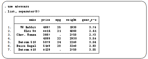
The data allow us to make some guesses at the values in the dataset, but, for example, we do not know the units in which the price or weight is measured, and the term “mpg” could be confusing for people outside the United States. Perhaps we can learn something from the description of the dataset. Stata has the aptly named describe command for this purpose (as we saw in [GSW] 1 Introducing Stata—sample session).

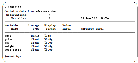
Though there is precious little information that could help us as a researcher, we can glean some information here about how Stata thinks of the data from the first three columns of the output.

1. The Variable name is the name we use to tell Stata about a variable.
2. The Storage type (otherwise known as the data type) is the way in which Stata stores the data in a variable. There are six different storage types, each having its own memory requirement:
   • For integers:

byte for integers between -127 and 100 (using 1 byte of memory per observation) int for integers between -32,767 and 32,740 (using 2 bytes of memory per observation) long for integers between -2,147,483,647 and 2,147,483,620 (using 4 bytes of memory per observation)

• • For real numbers:

float for real numbers with 8.5 digits of precision (using 4 bytes observation)

double for real numbers with 16.5 digits of precision (using 8 bytes observation)

• • For strings (text) between 1 and 2,045 bytes (using 1 byte of memory per character for ASCII and up to 4 bytes of memory per Unicode character):

str1 for 1-byte-long strings

str2 for 2-byte-long strings

str3 for 3-byte-long strings

…..

str2045 for 2,045-byte-long strings

• • Stata also has a strL storage type for strings of arbitrary length up to 2,000,000,000 bytes. strLs can also hold binary data, often referred to as BLOBs, or binary large objects, in databases. We will not illustrate these here.

Storage types affect both the precision of computations and the size of datasets. A quick guide to storage types is available at help data types or in [D] Data types.

3. The Display format controls how the variable is displayed; see [U] 12.5 Formats: Controlling how data are displayed. By default, Stata sets it to something reasonable given the storage type.

We would like to make this dataset into something containing all the information we need.

To see what a well-labeled dataset looks like, we can look at a dataset stored at the Stata Press repository. We need not load the data (and disturb what we are doing); we do not even need a copy of the dataset on our machine. (You will learn more about Stata’s Internet capabilities in [GSW] 19 Updating and extending Stata—Internet functionality.) All we need to do is direct describe to look at the proper file by using the command describe using filename.

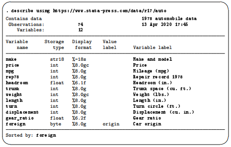
This output is much more informative. There are three locations where labels are attached that help explain what the dataset contains:

1. In the first line, 1978 automobile data is the data label. It gives information about the contents of the dataset. Data can be labeled by selecting Data > Data utilities > Label utilities > Label dataset, by using the label data command, or by editing the Label field in the Data portion of the Properties window. When doing this in the main window, be sure that the Properties window is unlocked.
2. There is a variable label attached to each variable. Variable labels are how we would refer to the variable in normal, everyday conversation. Here they also contain information about the units of the variables. Variables can be labeled by selecting the variable in the Variables window and editing the Label field in the Properties window. You can also change a variable label by using the Variables Manager or by using the label variable command.
3. The foreign variable has an attached value label. Value labels allow numeric variables such as foreign to have words associated with numeric codes. The describe output tells you that the numeric variable foreign has value label origin associated with it. Although not revealed by describe, the variable foreign takes on the values 0 and 1, and the value label origin associates 0 with Domestic and 1 with Foreign. If you browse the data (see [GSW] 6 Using the Data Editor), foreign appears to contain the values “Domestic” and “Foreign”. The values in a variable are labeled in two stages. The value label must first be defined. This can be done in the Data Editor, or in the Variables Manager, or by selecting Data > Data utilities > Label utilities>Manage value labels or by typing the label define command. After the labels have been defined, they must be attached to the proper variables, either by selecting Data > Data utilities>Label utilities > Assign value label to variables or by using the label values command.

Note: It is not necessary for the value label to have a name different from that of the variable. You could just as easily have used a value label named foreign.

3. Labeling datasets and variables

We will now load the afewcars.dta dataset and give it proper labels. We will do this with the Command window to illustrate that it is simple to do in this fashion. Earlier in Renaming and formatting variables in [GSW] 6 Using the Data Editor, we used the Data Editor to achieve a similar purpose. If you use the Data Editor for the material here, you will end up with the same commands in your log; we would like to illustrate a way to work directly with commands.

4. Labeling values of variables

We will now add a new indicator variable to the dataset that is 0 if the car was made in the United States and 1 if it was made in another country. Open the Data Editor and use your previously gained knowledge to add a foreign variable whose values match what is shown in this listing:

You can create this new variable in the Data Editor if you would like to work along. (See [GSW] 6 Using the Data Editor for help with the Data Editor.) Though the definitions of the categories “0” and “1” are clear in this context, it still would be worthwhile to give the values explicit labels because it will make output clear to people who are not so familiar with antique automobiles. This is done with a value label.

We saw an example of creating and attaching a value label by using the point-and-click interface available in the Data Editor in Changing data in [GSW] 6 Using the Data Editor. Here we will do it directly from the Command window.

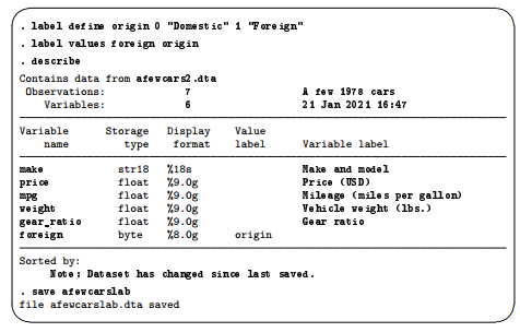
From this example, we can see that a value label is defined via

label define labelname # “contents” # “contents” .. .

It can then be attached to a variable via

label values variablename labelname

Once again, we need to save the dataset to be sure that we do not mistakenly lose the labels later. We saved this under a new filename because we have cleaned it up, and we would like to use it in the next chapter.

If you had wanted to define the value labels by using a point-and-click interface, you could do this with the Properties window in either the Main window or the Data Editor or by using the Variables Manager. See [GSW] 7 Using the Variables Manager for more information.

There is more to value labels than what was covered here; see [U] 12.6.3 Value labels for a complete treatment.

You may also add notes to your data and your variables. This feature was previously discussed in Renaming and formatting variables in [GSW] 6 Using the Data Editor and Managing notes in [GSW] 7 Using the Variables Manager. You can learn more about notes by typing help notes, or you can get the full story in [D] notes.

Source: STATA (2021), Getting Started with Stata for Windows, Stata Press Publication.