Monitoring the effort of team members in the firrm

In the light of the above, the individual employer under conditions of team production must therefore rely on monitoring to induce effort. We have already surmised in Chapter 4 that the proprietorship will be viable only if the returns to monitoring are ‘sufficiently great’. Again, to reinterpret this observation in the light of the analysis of Chapter 5 may be useful. Assume, as above, that there are only two effort levels, zero and e, which employees can choose. Assume further that if everyone chooses effort e the probabil­ity of outcome π will increase top₁^efrompy, otherwise the probability of will remain at pj.¹¹ Figure 5.5 can be reinterpreted to apply to the employer P and the ‘typical employee’ A, with indifference curves U_A^e now reflecting the utility index of the employee when the whole team is exerting effort e. If the employer could be absolutely certain of every employee’s effort simply by monitoring at a given level of intensity, the team would obviously be viable, providing the potential benefits, distance at, multiplied by the number of employees, exceeded the costs to the employer of the crit­ical level of monitoring required. Each employee would have a contract at a and would be monitored sufficiently intensely to determine with certainty that effort e was forthcoming. Providing the average monitoring cost per employee fell short of at, both employer and employee are capable of becoming better off than remaining at 0.

A natural extension of this analysis is to consider what would happen if the employer could observe the employee’s effort only with some accom­panying error. In section 5 it was shown how even a very ‘noisy’ signal could, in principle, improve the positions of both principal and agent.

However, in that section we were considering a case in which there existed a contract x involving the outcome alone which was Pareto preferred to the original position at θ in Figure 5.5. The addition of any informative, though noisy, signal could be used to improve further on such a contract. In the case here, however, we have assumed that no contract based on the outcome alone is viable, and our point of departure is from θ. Clearly, from this inauspicious starting point the principal’s information about the agent’s effort will have to be reasonably good if it is going to make much difference. Some signals may simply not be ‘informative enough’ to be capable of pro­viding opportunities for mutual benefit. On the other hand, intuition sug­gests that perfect information may not be necessary, and that a ‘sufficiently informative’ signal, which was nevertheless subject to error, might be useful.

That such a possibility exists can be seen by considering once more the monitoring gambles of section 5. There we saw that the labourer could, providing the monitor was more likely to observe ‘correctly’ than ‘incor­rectly’, be presented with a reward structure which implied that an idle labourer would be taking an ‘unfavourable’ gamble while an industrious labourer would be taking a ‘fair’ one. Now, unlike the labourer at point x in section 5, this will not be sufficient, in itself, to ensure that the labourer at a point such as a will prefer effort to no effort. The idle labourer at a will not like having to take an unfavourable gamble if he is monitored, but he does not like exerting effort e either, and the ‘effort price’ of avoiding the unfavourable gamble may be too high for him. (By contrast it will be recalled that at point x in the example of section 5, the labourer was indifferent between effort and no effort, so that there was no ‘effort price’ of avoiding the unfavourable gamble.)

Although the prospect of any unfavourable gamble will not automati­cally induce effort at point a, it is clearly possible that the prospect of an extremely unfavourable gamble might do the trick. At point a, the employee or agent would face the ‘monitoring gamble’:

assuming that effort zero were chosen. If the principal’s information is very good, so that both q_eo (that is, the probability of being observed working when the agent is in fact idle) and q_oe (the probability of being observed shirking when the agent is really working) are very small, the gamble m_A^a will be extremely unfavourable. Thus, the more reliable the information of the principal, the more adverse is the monitoring gamble taken by the shirker. It is at least possible to envisage a point at which work becomes more attractive than the monitoring gamble associated with idleness.

We cannot appeal to the limit theorem used in section 5 to prove this proposition, since it is clear that the ‘stakes’ cannot be infinitesimally small if the jump in effort from zero to e is to be forthcoming. The employee, or agent, will have to face values of S_e and S₀ sufficiently large to induce effort e whilst the value of π must be chosen so as to leave him as well off as he was at a. It is not, therefore, sufficient for the industrious labourer to be offered a ‘fair’ monitoring gamble at a, since risk-averse people will be made worse off by non-infinitesimal fair bets. The monitoring gamble will have to be favourable at a, or, if it is fair, the contract point must be to the right of a along A’s certainty line. In the latter case, providing a point exists to the left of t (say point p) where the agent is as well off exerting effort and taking a fair monitoring gamble as he was at θ, and providing the moni­toring gambles are so constructed that effort is preferred to idleness at p, the use of the principal’s less than completely reliable information may permit Pareto improvements on θ. Distance ap in Figure 5.5 represents the cost to the risk-averse agent of taking the fair monitoring bet. Clearly, other things constant, the bigger are S₀ and S_e the bigger will be the distance ap, but the more reliable the principal’s information the more adverse is the monitoring gamble of the shirker and the smaller can be the value of S₀ and S_e compatible with making effort the preferred option on the part of the agent. Thus, more reliable information will be associated with a smaller dis­tance ap.

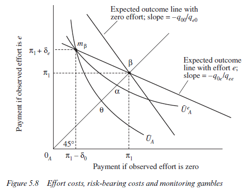
Figure 5.8 may help to illustrate the relationship between effort costs θa, risk-bearing costs ap, and the monitoring gambles. At point p, the agent receives ^ with certainty. This gives no incentive to exert effort. Now offer the agent a monitoring gamble, π + S_e, conditional upon being observed working, and π – S₀, conditional upon being observed idle. Further, ensure that this monitoring gamble is ‘fair’ for the industrious worker so ^that QeeK = %eh ^with Vee > ?fl*. Call this monitoring gamble point mp. Clearly, the agent will be worse off at mp than at p. The cost of bearing the uncertainty of the fair monitoring gamble is ap. For the idle labourer, however, fair gambles occur along the line through p slope -q₀₀/q_0e and hence the gamble at mp is clearly unfavourable. Draw the idle labourer’s indifference curve through mp and let it cut the certainty line at θ. If dis­tance θa is the cost to the agent of exerting effort level e, the agent will be indifferent at mp between effort and no effort; mp will represent the least costly monitoring gamble which is ‘fair’ to the industrious labourer and is just able to induce effort e.

The effect of more reliable information can now be deduced from the figure. An increase in q_oo/q_eo (that is, better information about the shirker) will steepen A’s indifference curve through θ. It follows that, at mp, A’s utility index will be lower than before if he shirks, and he will strictly prefer effort to no effort. Thus, a less costly monitoring gamble between mp and p can be found. Even perfect information about the shirker will not remove risk-bearing costs entirely, however, if there is a chance of perceiving an industrious labourer as idle. Zero risk-bearing costs would require perfect information about the industrious worker; that is, q_oe/q_ee = 0.

If we now introduce the complication that reliability of information may depend upon the monitoring costs incurred by the principal, we see that the distance pt in Figure 5.5 will exaggerate the gains to be had from monitor­ing by the amount of these costs. This suggests that there may be some efficient amount of monitoring effort on the part of the principal. At very low levels of monitoring effort, the information may be so unreliable that p lies to the right of point t and no Pareto improvement on θ is possible. At very high levels of monitoring effort, point p may lie close to point a. The risk-bearing costs associated with the monitoring gamble are low because information is very reliable, but in this case the monitoring costs may be so big that they more than absorb the potential benefits pt, and there is still no Pareto improvement on θ. If monitoring is to be viable, there must be a point at which the distance pt minus total monitoring costs is positive, and the efficient amount of monitoring effort will be that at which distance pt minus costs of monitoring is maximised. This gives us a new perspective on Figure 4.2 in Chapter 4. There we argued that monitoring effort would be applied to the point at which marginal benefits and costs were equal. Here we are looking behind the MB₁ schedule. The benefit of additional moni­toring in this framework is more reliable information. A given amount of effort e can thus be induced from each employee using monitoring gambles involving lower risk-bearing costs.

Source: Ricketts Martin (2002), The Economics of Business Enterprise: An Introduction to Economic Organisation and the Theory of the Firm, Edward Elgar Pub; 3rd edition.