Other Situation Sets of Experimental Research

Thus far we have dealt in detail with only, perhaps, the two most used situation sets. We have seen the difference of requiring the additional steps in the procedure for situations in which a is not known. This difference applies to all other situation sets as well. We will now visit a few more situation sets, some significantly different from the above two; for each we will mention the differ­ ence in the formulas used for computing N, the sample size X, the criterion value, and, further, the rules for accepting or reject­ing the hypotheses.

Situation Set 3

All the situations in this set are exactly the same as in Situation Set 1, with the only difference that the alternate hypothesis here is

Procedure:

The steps are like those for Situation Set 1; the difference is only in step (9), the criteria for accepting one of the hypotheses.

Calculate the criterion number:

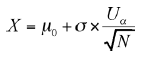
Then, after getting X1 the mean of the improved dependent variable,

10. Make the decision:

If X1 ≤ X, accept the alternate hypothesis, Hα: μ1 < μ0 with confidence of (1 – α) 100 percent or higher.

If X1 > X, accept the null hypothesis, H0: μ1 = μ0.

Situation Set 4

Example 4:

This is a test for the simple comparison of two populations, A and B: no experiment is involved.

This, unlike Situation Sets 1 and 2, is two sided, meaning it can be either μ1 > μ0 or μ1 < μ0.

μ0 and μ1 are both known.

1. σ, the standard deviations of the measurements used for both μ0 and μ1, is known.
2. NA and NB, the number of samples from the two populations, both are known.

Procedure:

2. State the hypotheses:

Alternate hypothesis: Hα: μ1 ≠ μ0

3. Choose ρ (similar to α and β), the risk factor. This, like in Situation Set 1, is a subjective judg­ment made by the experimenter.
4. Go to Table 18.3, which gives the probability points U for the above set of situations.

Corresponding to ρ chosen, find Uρ.

6. Calculate the criterion number.

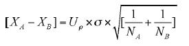
10.  Follow the rules:

1. 1. If [XA – XB] is a positive number, accept the alternate hypothesis, Hα1: μA > μB, with a confidence of (1 – α/2) × 100 percent or more.
   2. If [XA – XB] is a negative number, accept the alternate hypothesis, H2a: μA < μB, with a confidence of (1 – α/2) × 100 percent or more.
   3. If [XA – XB] is zero, accept the null hypothesis, H0: μA = μB, with a confidence of (1 – β) × 100 percent or more.

Situation Set 5

All conditions in this set are exactly like those in Situation Set 4, with the only exception that O1 ^ O2, though both O1 and O2 are known.

6. Then, the criterion number is given by

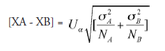
The decisions on accepting and rejecting the hypothesis, based on the criterion number, are the same as in Situation Set 4.

Situation Set 6

The same specimen (or a part or a person) is measured for a given property (or capacity or performance) (1) before and (2) after improvement. Several such specimens, together, constitute the subjects for the experiment. Examples of such situations are (1) the effect of hardening heat treatment on a given alloy, (2) a new drug being tested for lowering the blood pressure of hypertension patients, and (3) the kick length of a soccer ball tested for a group of players before and after they take a miracle drink. The differ­ence in property (or capacity or performance), symbolized by fj), is the population under consideration.

Example 5:

Each of the twenty-seven players on a high school soccer team are made to kick the soccer ball three times; the longest kick of each player is recorded as an element in the first sample. Each player is then given a measured quantity of a miracle drink. Ten minutes after taking the drink, the same twenty-seven players are made to repeat the performance of kicking the ball; the sec­ond sample, with a similar procedure as for the first, is collected from this repetition.

Procedure:

1. It is considered reasonable in such situations to assume the numerical value of O to be the same as that of 8; hence, the question as to whether O is known or unknown disappears.
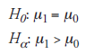
2. State the hypotheses:

3. Choose α and β.
4. Look up for Uα and Uβ (one sided, Table 18.2).

5. Compute Ni, the sample size:

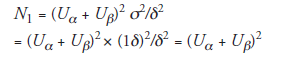
5a. Find the degree of freedom, given by F = (N1 — 1).

(3)2.      Look for t-values for <Φ(one sided, Table 18.4).

Second iteration:

⁽⁵⁾2       

1. Experiment with N2 sample items.
2. Find (Xβ – Xα), the difference between Xβ, the lengths of the kick after taking the miracle drink, and Xα,the corresponding length before taking the drink, for each one of the randomly selected N2 players.
3. Find X1, the mean of the N2 of such (Xβ – Xα) values:

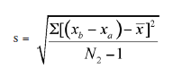
(1)2. Find s, the estimated standard deviation for N2 measures of (Xb – Xa):

(5a)2. Find the degree of freedom, second iteration: Φ2 = N2 – 1.
3. Find tα for Φ2 (one sided, Table 18.4).
6. Compute the criterion value,
9. Compare X, and X, and
10. Make the decsion:

9 and 10. Compare X1 and X, and make the decision:\

If X1 > X, accept the alternate hypothesis with (1 – α) × 100 percent confidence.

If X1 < X, accept the null hypothesis.

Source: Srinagesh K (2005), The Principles of Experimental Research, Butterworth-Heinemann; 1st edition.