In this section, we discuss a supply chain design decision at D-Solar, a German manufacturer of solar panels, to illustrate the power of the decision tree analysis methodology for designing global supply chain networks while accounting for uncertainty. D-Solar faces a plant location decision in a global network with fluctuating exchange rates and demand uncertainty.
1. Key Point
Flexibility should be valued by taking into account uncertainty in demand and economic factors. In general, the value of flexibility increases with an increase in uncertainty.
D-Solar sells its products primarily in Europe. Demand in the Europe market is currently 100,000 panels per year, and each panel sells for €70. Although panel demand is expected to grow, there are some downside risks if the economy slides. From one year to the next, demand may increase by 20 percent, with probability 0.8, or decrease by 20 percent, with probability 0.2.
D-Solar has to decide whether to build a plant in Europe or China. In either case, D-Solar plans to build a plant with a rated capacity of 120,000 panels. The fixed and variable costs of the two plants are shown in Table 6-12. Observe that the fixed costs are given per year rather than as a one-time investment. The European plant is more expensive but will also have greater volume flexibility. The plant will be able to increase or decrease production anywhere in the range of 60,000 to 150,000 panels while maintaining its variable cost. In contrast, the Chinese plant is cheaper (at the current exchange rate of 9 yuan/euro) but will have limited volume flexibility and can produce only between 100,000 and 130,000 panels. If the Chinese plant is built, D-Solar will have to incur variable cost for 100,000 panels even if demand drops below that level and will lose sales if demand increases above 130,000 panels. Exchange rates are volatile; each year, the yuan is expected to rise 10 percent, with a probability of 0.7, or drop 10 percent, with a probability of 0.3. We assume that the sourcing decision will be in place over the next three years and the discount rate used by D-Solar is k = 0.1. All costs and revenues are assumed to accrue at the beginning of the year, allowing us to consider the first year as period 0 and the following two years as periods 1 and 2.

2. Evaluating the Options Using Expected Demand and Exchange Rate
A simplistic approach often taken is to consider the expected movement of demand and exchange rates in future periods when evaluating discounted cash flows. The weakness of such an approach is that it averages the trends while ignoring the uncertainty. We start by considering such a simplistic approach for the onshoring and offshoring options. On average, demand is expected to increase by 12 percent [(20 X 0.8) – (20 X 0.2) = 12], whereas the yuan is expected to strengthen by 4 percent [(10 X 0.7) – (10 X 0.3) = 4] each year. The expected demand and exchange rates in the two future periods are shown in Table 6-13.
We now evaluate the discounted cash flows for both options assuming the average expected change in demand and exchange rates over the next two periods.
For the onshoring option, we have the following:
Period 0 profits = (100,000 X 70) – 1,000,000 – (100,000 X 40) = € 2,000,000
Period 1 profits = (112,000 X 70) – 1,000,000 – (112,000 X 40) = €2,360,000
Period 2 profits = (125,440 X 70) – 1,000,000 – (125,440 X 40) = €2,763,200
Thus, the DCF for the onshoring option is obtained as follows:
Expected profit from onshoring = 2,000,000 + 2,360,000/ 1.1 + 2,763,200/ 1.21 = €6,429,091

For the offshoring option, we have the following:
Period 0 profits = (100,000 X 70) – (8,000,000/ 9) – (100,000 X 340/ 9) = €2,333,333
Period 1 profits = (112,000 X 70) – (8,000,000 / 8.64) – (112,000 X 340 / 8.64) = € 2,506,667
Period 2 profits = (125,440 X 70) – (8,000,000 / 8.2944) – (125,440 X 340/ 8.2944) = € 2,674,319
Thus, the DCF for the offshoring option is obtained as follows:
Expected profit from offshoring = 2,333,333 + 2,506,667 / 1.1 + 2,674,319 / 1.21 = €6,822,302
Based on performing a simple DCF analysis and assuming the expected trend of demand and exchange rates over the next two periods, it seems that offshoring should be preferred to onshoring because it is expected to provide additional profits of almost €393,000.
The problem with the preceding analysis is that it has ignored uncertainty. For example, even though the demand is expected to grow, there is some probability that it will decrease. If demand drops below 100,000 panels, the offshore option could end up costing more because of the lack of flexibility. Similarly, if demand increases more than expected (for example, if it grows by 20 percent in each of the two years), the offshore facility will not be able to keep up with the increase. An accurate analysis must reflect the uncertainties and should ideally be performed using a decision tree.
3. Evaluating the Options Using Decision Trees
For this analysis we construct a decision tree, as shown in Figure 6-3. Each node in a given period leads to four possible nodes in the next period because demand and the exchange rate may go up or down. The detailed links and transition probabilities are shown in Figure 6-3. Demand is in thousands and is represented by D. The exchange rate is represented by E, where E is the number of yuan to a euro. For example, starting with the node D = 100, E = 9.00 in Period 0, one can transition to any of four nodes in Period 1. The transition to the node D = 120, E = 9.90 in Period 1 occurs if demand increases (probability of 0.8) and the yuan weakens (probability of 0.3). Thus, the transition from node D = 100, E = 9.00 in Period 0 to node D = 120, E = 9.90 in Period 1 occurs with probability 0.8 X 0.3 = 0.24. All other transition probabilities in Figure 6-3 are calculated in a similar manner. The main advantage of using a decision tree is that it allows for the true evaluation of profits in each scenario that D-Solar may find itself.
4. Evaluating the onshore option
Recall that the onshore option is flexible and can change production levels (and thus variable costs) to match demand levels between 60,000 and 150,000. In the following analysis, we calculate the expected profits at each node in the decision tree (represented by the corresponding values of D and E) starting in Period 2 and working back to the present (Period 0). With the onshore option, exchange rates do not affect profits in euro because both revenue and costs are in euro.
PERIOD 2 EVALUATION We provide a detailed analysis for the node D = 144 (solar panel demand of 144,000), E = 10.89 (exchange rate of 10.89 yuan per euro). Given its flexibility, the onshore facility is able to produce the entire demand of 144,000 panels at a variable cost of €40 and sell each panel for revenue of €70. Revenues and costs are evaluated as follows:
Revenue from the manufacture and sale of 144,000 panels
= 144,000 X 70 = €10,080,000
Fixed + variable cost of onshore plant = 1,000,000 + (144,000 X 40)
= €6,760,000

In Period 2, the total profit for D-Solar at the node D = 144, E = 10.89 for the onshore option is thus given by
P(D = 144, E = 10.89, 2) = 10,080,000 – 6,760,000 = €3,320,000
Using the same approach, we can evaluate the profit in each of the nine states (represented by the corresponding value of D and E) in Period 2, as shown in Table 6-14.
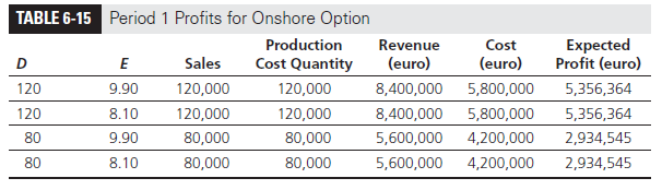
PERIOD 1 EVALUATION Period 1 contains four outcome nodes to be analyzed. A detailed analysis for one of the nodes, D = 120, E = 9.90, is presented here. In addition to the revenue and cost at this node, we also need to consider the present value of the expected profit in Period 2 from the four nodes that may result. The transition probability into each of the four nodes is as shown in Figure 6-3. The expected profit in Period 2 for the four potential outcomes resulting from the node D = 120, E = 9.90 is thus given by
EP{D = 120, E = 9.90, 1) = 0.24 X P(D = 144, E = 10.89, 2) + 0.56 X P(D = 144, E = 8.91,2) + 0.06 X P(D = 96, E = 10.89, 2) + 0.14 X P(D = 96, E
= 8.91, 2) = (0.24 X 3,320,000) + (0.56 X 3,320,000)+ (0.06 X 1,880,000) + (0.14 X 1,880,000)
= €3,032,000

The present value of the expected profit in Period 2 discounted to Period 1 is given by
PVEP( D = 120, E = 9.90, 1) = EP(D = 120, E = 9.90, 1)/(1 + k)
= 3, 032,000 / 1.1 = €2, 756,364
Next we evaluate the profits at the onshore plant at the node D = 120, E = 9.90 from its operations in Period 1, in which the onshore plant produces 120,000 panels at a variable cost of €40 and obtains revenue of €70 per panel. Revenues and costs are evaluated as follows:
Revenue from manufacture and sale of 120,000 panels
= 120,000 X 70 = € 8,400,000
Fixed + variable cost of onshore plant = 1,000,000 + (120,000 X 40)
= €5,800,000
The expected profit for D-Solar at the node D = 120, E = 9.90 is obtained by adding the operational profits at this node in Period 1 and the discounted expected profits from the four nodes that may result in Period 2. The expected profit at this node in Period 1 is given by
P(D = 120, E = 9.90, 1) = 8,400,000 – 5,800,000 + PVEP(D = 120, E = 9.90, 1)
= 2,600,000 + 2,756,364 = € 5,356,364
The expected profits for all nodes in Period 1 are calculated similarly and shown in Table 6-15.
PERIOD 0 EVALUATION In Period 0, the demand and exchange rate are given by D = 100, E = 9. In addition to the revenue and cost at this node, we also need to consider the discounted expected profit from the four nodes in Period 1. The expected profit is given by
EP(D = 100, E = 9.00, 0) = 0.24 X P(D = 120, E = 9.90, 1) + 0.56 X P(D = 120, E = 8.10, 1) + 0.06 X P(D = 80, E = 9.90, 1) + 0.14 X P(D = 80, E = 8.10, 1)
= (0.24 X 5,356,364) + (0.56 X 5,356,364) + (0.06 X 2,934,545) + (0.14 X 2,934,545)
= €4,872,000
The present value of the expected profit in Period 1 discounted to Period 0 is given by
PVEP(D = 100, E = 9.00, 0) = EP(D = 100, E = 9.00, 0) / (1 + k)
= 4,872,000 / 1.1 = €4,429,091
Next, we evaluate the profits from the onshore plant’s operations in Period 0 from the manufacture and sale of 100,000 panels.
Revenue from manufacture and sale of 100,000 panels
= 100,000 X 70 = €7,000,000
Fixed + variable cost of onshore plant = 1,000,000 + (100,000 X 40)
= € 5,000,000
The expected profit for D-Solar at the node D = 100, E = 9.00 in Period 0 is given by
P(D = 100, E = 9.00, 0) = 7,000,000 – 5,000,000 + PVEP(D = 100, E = 9.00, 0)
= 2,000,000 + 4,429,091 = €6,429,091
Thus, building the onshore plant has an expected payoff of €6,429,091 over the evaluation period. This number accounts for uncertainties in demand and exchange rates and the ability of the onshore facility to react to these fluctuations.
5. Evaluating the Offshore Option
As with the onshore option, we start by evaluating profits at each node in Period 2 and then back our evaluation up to Periods 1 and 0. Recall that the offshore option is not fully flexible and can change production levels (and thus variable costs) only between 100,000 and 130,000 panels. Thus, if demand falls below 100,000 panels, D-Solar still incurs the variable production cost of 100,000 panels. If demand increases above 130,000 panels, the offshore facility can meet demand only up to 130,000 panels. At each node, given the demand, we calculate the expected profits accounting for the exchange rate that influences offshore costs evaluated in euro.
PERIOD 2 EVALUATION The detailed analysis for the node D = 144 (solar panel demand of 144,000), E = 10.89 (exchange rate of 10.89 yuan per euro) is as follows. Even though demand is for 144,000 panels, given its lack of volume flexibility, the offshore facility is able to produce only 130,000 panels at a variable cost of 340 yuan each and sell each panel for a revenue of €70. Revenues and costs are evaluated as follows:
Revenue from manufacture and sale of 130,000 panels
= 130,000 X 70 = €9,100,000
Fixed + variable cost of offshore plant = 8,000,000 + (130,000 X 340)
= 52,200,000 yuan
The total profit for D-Solar at the node D = 144, E = 10.89 for the offshore option (evaluated in euro), is thus given by
P(D = 144, E = 10.89, 2) = 9, 100, 000 – (52, 200, 00/10.89) = €4,306,612
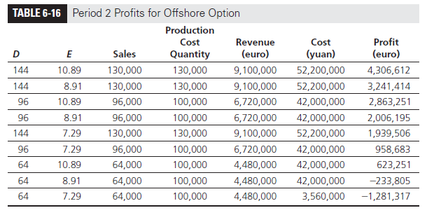
Using the same approach, we can evaluate the profit in each of the nine states (represented by the corresponding values of D and E) in Period 2 as shown in Table 6-16. Observe that the lack of flexibility at the offshore facility hurts D-Solar whenever demand is above 130,000 (lost margin) or below 100,000 (higher costs). For example, when the demand drops to 64,000 panels, the offshore facility continues to incur variable production costs for 100,000 panels. Profits are also hurt when the yuan is stronger than expected.
PERIOD 1 EVALUATION In Period 1, there are four outcome nodes to be analyzed. As with the onshore option, a detailed analysis for the node D = 120, E = 9.90 is presented here. In addition to the revenue and cost from operations at this node, we also need to consider the present value of the expected profit in Period 2 from the four nodes that may result. The transition probability into each of the four nodes is as shown in Figure 6-3. The expected profit in Period 2 from the node D = 120, E = 9.90 is thus given by
EP(D = 120, E = 9.90, 1) = 0.24 X P(D = 144, E = 10.89, 2) + 0.56 X P(D = 144, E = 8.91,2) + 0.06 X P(D = 96, E = 10.89, 2) + 0.14 X P(D = 96, E = 8.91, 2)
= (0.24 X 4,306,612) + (0.56 X 3,241,414)+ (0.06 X 2,863,251) + (0.14 X 2,006,195)
= €3,301,441
The present value of the expected profit in Period 2 discounted to Period 1 is given by
PVEP( D = 120, E = 9.90, 1) = EP(D = 120, E = 9.90, 1) / (1 + k)
= 3,301, 441 / 1.1 = € 3,001,310
Next, we evaluate the profits at the offshore plant at the node D = 120, E = 9.90 from its operations in Period 1. The offshore plant produces 120,000 panels at a variable cost of 340 yuan and obtains revenue of €70 per panel. Revenues and costs are evaluated as follows:
Revenue from manufacture and sale of 120,000 panels
= 120,000 X 70 = € 8,400,000
Fixed + variable cost of onshore plant = 8,000,000 + (120,000 X 340)
= 48,800,000 yuan
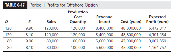
The expected profit for D-Solar at the node D = 120, E = 9.90 in Period 1 is given by
P(D = 120, E = 9.90, 1) = 8,400,000 – (48,800,00 /9.90) + PVEP(D = 120, E = 9.90, 1)
= 3,470,707 + 3,001,310 = € 6,472,017
For the offshore option, the expected profits for all nodes in Period 1 are shown in Table 6-17.
Observe that for the node D = 80, E = 8.10, D-Solar has a lower expected profit from the offshore option (Table 6-17) relative to the onshore option (see Table 6-15) because the offshore plant incurs high variable cost, given its lack of flexibility (cost is incurred for 100,000 units even though only 80,000 are sold), and all offshore costs become expensive, given the strong yuan.
PERIOD 0 EVALUATION In Period 0, the demand and exchange rate are given by D = 100, E = 9.
In addition to the revenue and cost at this node, we also need to consider the present value of expected profit from the four nodes in Period 1. The expected profit for the offshore option is given by
EP(D = 100, E = 9.00, 0) = 0.24 X P(D = 120, E = 9.90, 1) + 0.56 X P(D = 120, E = 8.10, 1) + 0.06 X P(D = 80, E = 9.90, 1) + 0.14 X P(D = 80, E = 8.10, 1)
= (0.24 X 6,472,017) + (0.56 X 4,301,354)+ (0.06 X 3,007,859) + (0.14 X 1,164,757)
= € 4,305,580
The present value of the expected profit in Period 1 discounted to Period 0 is given by
PVEP(D = 100, E = 9.00, 0) = EP(D = 100, E = 9.00, 0) / (1 + k)
= 4,305,580 / 1.1 = € 3,914,164
Next we evaluate the profits from the offshore plant’s operations in Period 0 from the manufacture and sale of 100,000 panels.
Revenue from manufacture and sale of 100,000 panels
= 100,000 X 70 = € 7,000,000
Fixed + variable cost of offshore plant = 8,000,000 + (100,000 X 340)
= 42,000,000 yuan
The expected profit for D-Solar at the node D = 100, E = 9.00 in Period 0 is given by
P(D = 100, E = 9.00, 0) = 7,000,000 – (42,000,00 / 9.00) + PVEP(D = 100, E = 9.00, 0)
= 2,333,333 + 3,914,164 = € 6,247,497
Thus, building the offshore plant has an expected payoff of €6,247,497 over the evaluation period.
Observe that the use of a decision tree that accounts for both demand and exchange rate fluctuation shows that the onshore option, with its flexibility, is in fact more valuable (worth €6,429,091) than the offshore facility (worth €6,247,497), which is less flexible. This is in direct contrast to the decision that would have resulted if we had simply used the expected demand and exchange rate for each year. When using the expected demand and exchange rate, the onshore option provided expected profits of €6,429,091, whereas the offshore option provided expected profits of €6,822,302. The offshore option is overvalued in this case because the potential fluctuations in demand and exchange rates are wider than the expected fluctuations. Using the expected fluctuation thus does not fully account for the lack of flexibility in the offshore facility and the big increase in costs that may result if the yuan strengthens more than the expected value.
De Treville and Trigeorgis (2010) discuss the importance of evaluating all global supply chain design decisions using the decision tree or real options methodology. They give the example of Flexcell, a Swiss company that offered lightweight solar panels. In 2006, the company was looking to expand its operations by building a new plant. The three locations under discussion were China, eastern Germany, and near the company headquarters in Switzerland. Even though the Chinese and eastern German plants were cheaper than the Swiss plant, Flexcell management justified building the high-cost Swiss plant because of its higher flexibility and ability to react to changing market conditions. If only the expected values of future scenarios had been used, the more expensive Swiss plant could not be justified. This decision paid off for the company because the Swiss plant was flexible enough to handle the considerable variability in demand that resulted during the downturn in 2008.
When underlying decision trees are complex and explicit solutions for the underlying decision tree are difficult to obtain, firms should use simulation for evaluating decisions (see Chapter 13). In a complex decision tree, thousands or even millions of possible paths may arise from the first period to the last. Transition probabilities are used to generate probability- weighted random paths within the decision tree. For each path, the stage-by-stage decision and the present value of the payoff are evaluated. The paths are generated in such a way that the probability of a path being generated during the simulation is the same as the probability of the path in the decision tree. After generating many paths and evaluating the payoffs in each case, the payoffs obtained during the simulation are used as a representation of the payoffs that would result from the decision tree. The expected payoff is then found by averaging the payoffs obtained in the simulation.
Source: Chopra Sunil, Meindl Peter (2014), Supply Chain Management: Strategy, Planning, and Operation, Pearson; 6th edition.
There is certainly a great deal to know about this subject.
I like all of the points you made.
I have been surfing online more than 3 hours these days, but I by no means found any interesting article like yours. It is pretty price enough for me. Personally, if all website owners and bloggers made excellent content as you did, the net will be much more useful than ever before.