Practicing Non-Parametric Tests in the Research

Non-parametric tests use statistics (that is, calculations) that have been estab­lished from observations, and do not depend on the distribution of the cor­responding population. The validity of non-parametric tests depends on very general conditions that are much less restrictive than those that apply to para­metric tests.

Non-parametric tests present a number of advantages, in that they are applicable to:

• small samples
• various types of data (nominal, ordinal, intervals, ratios)
• incomplete or imprecise data.

1. Testing One Variable in Several Samples

1.1. Comparing a distribution to a theoretical distribution: goodness-of-fit test

Research question Does the empirical distribution D_e, observed in a sample, differ significantly from a reference distribution D_r?

Application conditions

• The sample is random and contains n independent observations arranged into k
• A reference distribution, D_r, has been chosen (normal distribution, Chi- square, etc.).

Hypotheses

Null hypothesis, H₀: D_e = D_r,

alternative hypothesis, H₁: D_e # D_r

Statistic

The statistic calculated is

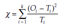
where, for each of the k classes, O_t is the number of observations made on the sample and T_t is the theoretical number of observations calculated according to the reference distribution D_r.

The statistic c follows a chi-square distribution with k – 1 – r degrees of free­dom, where r is the number of parameters of the reference distribution that have been estimated with the aid of observations.

Interpreting the test The decision rule is the following:

H₀ will be rejected if

1.2. Comparing the distribution of a variable X in two populations (Kolmogorov-Smirnov test)

Research question Is the variable X distributed identically in two populations, A and B?

The Kolmogorov-Smirnov test may also be used to compare an observed distribution to a theoretical one.

Application conditions

• The two samples are random and contain n_A and n_B independent observa­tions, taken from populations A and B
• The variable X is an interval or a ratio variable of any distribution.
• The classes are defined in the same way in both samples.

Hypotheses

Null hypothesis, H₀: The distribution of variable X is identical in A and B, alternative hypothesis, H₁: The distribution of variable X is different in A and B.

Statistic

The statistic calculated is:

where FA(x) and FB(x) represent the cumulated frequencies of the classes in A and in B. These values are compared to the critical values d₀ of the Kolmogorov-Smirnov table.

Interpreting the test The decision rule is the following: H₀ will be rejected if d > d₀.

1.3. Comparing the distribution of a variable X in two populations: Mann-Whitney U test

Research question Is the distribution of the variable X identical in the two populations A and B?

Application conditions

• The two samples are random and contain n_A and n_B independent observa­tions from populations A and B respectively (where n_A > n_B). If required, the notation of the samples may be inverted.
• The variable X is ordinal.

Hypotheses

Null hypothesis, H₀: The distribution of the variable X is identical in A and B, alternative hypothesis, Hp The distribution of the variable X is different in A and B.

Statistic

(A₁, A₂, …, A_nA) is a sample, of size n_A, selected from population A, and (B₁, B₂, …, B_nB) is a sample of size n_B selected from population B. N = n_A + n_B observations are obtained, which are classed in ascending order regardless of the samples they are taken from. Each observation is then given a rank: 1 for the smallest value, up to N for the greatest.

The statistic calculated is:

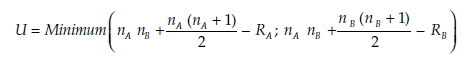
where R_A is the sum of the ranks of the elements in A, and R_B the sum of the ranks of the elements in B. The statistic U is compared to the critical values U_a of the Mann-Whitney table.

Interpreting the test The decision rule is the following: H₀ will be rejected if U < U_a.

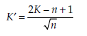
For large values of n_A and n_B (that is, > 12),

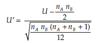
tends rapidly toward a standard normal distribution. U’ may then be used, in association with the decision rules of the standard normal distribution for rejecting or not rejecting the null hypothesis.

1.4. Comparing the distribution of a variable X in two populations: Wilcoxon test

Research question Is the distribution of the variable X identical in the two populations A and B?

Application conditions

• The two samples are random and contain n_A and n_B independent observa­tions from populations A and B
• The variable X is at least ordinal.

Hypotheses

Null hypothesis, H₀: The distribution of variable X is identical in A and B, alternative hypothesis, H₁: The distribution of variable X is different in A and B.

Statistic

(A₁, A₂, …, A_nA) is a sample, of size n_A, selected from population A, and (B₁, B₂, …, B_nB) is a sample of size n_B selected from population B. N = n_A + n_B observations are obtained, which are classed in ascending order regardless of the samples they are taken from. Each observation is then given a rank: 1 for the smallest value, up to N for the greatest.

The statistic calculated is:

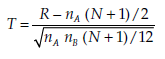
where R(A) is the rank of observation A_;, i = 1,2, …, nA and

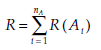
the sum of all the ranks of the observations from sample A.

The statistic T is compared to critical values R_a available in a table.

Interpreting the test The decision rule is the following:

H₀ will be rejected if R < R_a.

If N is sufficiently large (that is, n > 12), the distribution of T approximates a standard normal distribution, and the corresponding decision rules apply, as described above. When a normal distribution is approximated, a mean rank can be associated with any equally placed observations, and the formula becomes:

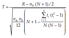
where g is the number of groups of equally-placed ranks and t_t is the size of group i.

1.5. Comparing variable distribution in two populations: testing homogenous series

Research question Is the distribution of the variable X identical in the two populations A and B?

Application conditions

• The two samples are random and contain n_A and n_B independent observa­tions from the populations A and B
• The variable X is at least ordinal.

Hypotheses

Null hypothesis, H₀: The distribution of the variable X is identical in A and B, alternative hypothesis, H₁: The distribution of the variable X is different in A and B.

Statistic

(A₁, A₂, … , A_nA) is a sample, of size n_A, selected from population A, and (B₁, B₂, …, B_nB) is a sample of size n_B selected from population B. N = n_A + n_B obser­vations are obtained, which are classed in ascending order regardless of the samples they are taken from. Each observation is then given a rank: 1 for the smallest value, up to N for the greatest.

The statistic calculated is:

R = the longest ‘homogenous series’ (that is, series of consecutive values belong­ing to one sample) found in the general series ranking the n_A + n_B observations. The statistic R is compared to critical values C_a available in a table.

Interpreting the test The decision rule is the following:

H₀ will be rejected if R < C_a.

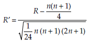
For large values of n_A and n_B (that is, > 20),

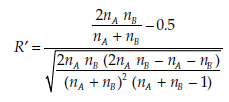
tends towards the standard normal distribution. R’ may then be used instead, in association with the decision rules of the standard normal distribution for rejecting or not rejecting the null hypothesis.

1.6. Comparing the distribution of a variable X in k populations: Kruskal-Wallis test or analysis of variance by ranking

Research question Is the distribution of the variable X identical in the k popu­lations A₁, A₂, … , A_k?

Application conditions

• The two samples are random and contain n₁, n₂,… n_k independent observa­tions from the populations A_v A₂, … A_k.
• The variable X is at least ordinal.

Hypotheses

Null hypothesis, H₀: The distribution of the variable X is identical in all k populations,

alternative hypothesis, Hp The distribution of the variable X is different in at least one of the k populations.

Statistic

(A_u, A₁₂, … , A_1n1) is a sample of size n₁ selected from population A_k and (A₂₁, A₂₂, … , A_2n2) is a sample of size n₂ selected from population A₂.

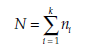
observations are obtained, which are classed in ascending order regardless of the samples they are taken from. Each observation is then given a rank: 1 for the smallest value, up to N for the greatest. For equal observations, a mean rank is attributed. R_t is the sum of the ranks attributed to observations of sample A.

The statistic calculated is:

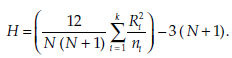
If a number of equal values are found, a corrected value is used:

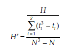
where g is the number of groups of equal values, and t_i the size of group i. Interpreting the test The decision rule is the following:

H₀ will be rejected if H (or, the case being, H’) >%2 __{a; k} _ ₁ or a corresponding value in the Kruskal-Wallis table.

If the Kruskal-Wallis test leads to the rejection of the null hypothesis, it is possible to identify which pairs of populations tend to be different. This requires the application of either the Wilcoxon signed test or the sign test if the samples are matched (that is, logically linked, such that the pairs or n-uplets of observations in the different samples contain identical or similar individuals), or a Mann-Whitney U or Wilcoxon test if the samples are not matched. This is basically the same logic as used when associating the analysis of variance and the LSD test. The Mann-Whitney U is sometimes called analysis of variance by rank.

1.7. Comparing two proportions or percentages (small samples)

Research question Do the two proportions or percentages p₁ and p₂, observed in two samples, differ significantly from each other?

Application conditions

• The two samples are random and contain n₁ and n₂ independent observa­tions respectively.
• The size of the samples is small (n₁ < 30 and n₂ < 30).
• The two proportions p₁ and p₂ as well as their complements 1-p₁ and 1-p₂ represent at least 5 observations.

Hypotheses

Null hypothesis, H₀: π₁ = π₂, alternative hypothesis, H₁: π₁ # π₂

Statistic

The statistic calculated is

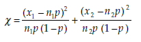
where x₁ is the number of observations in sample 1 (size n₁) corresponding to the proportion p₁, X₂ is the number of observations in sample 2 (size n₂) corre­sponding to the proportion p₂, and

This statistic % follows a chi-square distribution with 1 degree of freedom.

Interpreting the test The decision rule is the following:

H₀ will be rejected if x > x2a1

2. Tests on More than One Variable in One or Several Matched Samples

Two or more samples are called matched when they are linked in a logical man­ner, and the pairs or n-uplets of observations of different samples contain iden­tical or very similar individuals. For instance, samples comprised of the same people observed at different moments in time may comprise as many matched samples as observation points in time. Similarly, a sample of n individuals and another containing their n twins (or sisters, brothers, children, etc.) may be made up of matched samples in the context of a genetic study.

2.1. Comparing any two variables: independence or homogeneity test

Research question Are the two variables X and Y independent?

Application conditions

• The sample is random and contains n independent observations.
• The observed variables X and Y may be of any type (nominal, ordinal, inter­val, ratio) and are illustrated by k_X and k_Y

Hypotheses

Null hypothesis, H₀: X and Y are independent, alternative hypothesis, H₁: X and Y are dependent

Statistic

The statistic calculated is

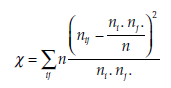
where n_i, designates the number of observations presenting both characteristics X_t and Y, (i varying from 1 to k_X; j from 1 to k_Y),

is the number of observations presenting the characteristics X_i and

is the number of observations presenting the characteristics X_j.

This statistic % follows a chi-square distribution with (k_X – 1) (k_Y – 1) degrees of freedom.

Interpreting the test The decision rule is the following:

^H0 ^WiH ^{be rejected if} x > x²_a.₍k_X _ 1) (y _ 1)

2.2. Comparing two variables X and Y measured from two matched samples A and B: sign test

Research question Are the two variables X and Y, measurable for two matched samples A and B, identically distributed?

Application conditions

• The two samples are random and matched.
• The n pairs of observations are independent.
• The variables X and Y are at least ordinal.

Hypotheses

Null hypothesis, H₀: The distribution of the two variables is identical in the two matched samples,

alternative hypothesis, H₁: The distribution of the two variables is different in the two matched samples.

Statistic

The pairs (a₁, b₁), (a₂, b₂), … , (a_n, b_n) are n pairs of observations, of which the first element is taken from population A and the second from population B. The difference a_t – b_t is calculated for each of these n pairs of observations (a, b). The number of positive differences is represented by k+, and the number of nega­tive differences by k-. The statistic calculated is:

K = Minimum (k+, k-).

The statistic K is compared to critical values C_a available in a table.

Interpreting the Test The decision rule is the following:

H₀ will be rejected if K < C_a.

For sufficiently large values of n (that is, n > 40),

tends towards the standard normal distribution. K’ may then be used instead, in association with the decision rules of the standard normal distribution for rejecting or not rejecting the null hypothesis.

2.3. Comparing variables from matched samples: Wilcoxon sign test

Research question Are the two variables X and Y, measured from two matched samples A and B, identically distributed?

Application conditions

• The two samples are random and matched.
• The n pairs of observations are independent.
• The variables X and Y are at least ordinal.

Hypotheses

Null hypothesis, H₀: The distribution of the two variables is identical in the two matched samples,

alternative hypothesis, Hp The distribution of the two variables is different in the two matched samples.

Statistic

(a₁, bj), (a₂, b₂), … , (a_n, b_n) are n pairs of observations, of which the first element is taken from the population A and the second from the population B. For each pair of observations, the difference d_t = a_t – b_t is calculated. In this way n dif­ferences d_i are obtained, and these are sorted in ascending order. They are ranked from 1, for the smallest value, to n, for the greatest. For equal-value rankings, a mean rank is attributed. Let R+ be the sum of the positive differ­ences and R— the sum of the negative ones.

The statistic calculated is:

R = Minimum (R+, R-)

The statistic R is compared to critical values R_a available in a table.

Interpreting the test The decision rule is the following: H₀ will be rejected if R < R_a.

For large values of n (that is, n > 20),

tends towards a standard normal distribution. R’ may then be used in associa­tion with the decision rules of the standard normal distribution for rejecting or not rejecting the null hypothesis.

2.4. Comparing variables from matched samples: Kendall rank correlation test

Research question Are the two variables, X and Y, measured for two matched samples A and B, independent?

Application conditions

• The two samples are random and matched.
• The n pairs of observations are independent.
• The variables X and Y are at least ordinal.

Hypotheses

Null hypothesis, H₀: X and Y are independent, alternative hypothesis, H₁: X and Y are dependent.

Statistic

The two variables (X, Y) observed in a sample of size n give n pairs of obser­vations (X₁, Y₁), (X₂, Y₂), … , (X_n, Y_n). An indication of the correlation between
variables X and Y can be obtained by sorting the values of X_i in ascending order and counting the number of corresponding Y_i values that do not respect this order. Sorting the values in ascending order guarantees that X_i < Xj for any value of i < j.

Let R be the number of pairs (X_i, Y.) such that, if i < j, X_i < Xj and Y_i < Y.

The statistic calculated is:

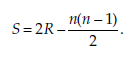
The statistic S is then compared to critical values S_a available in a table. Interpreting the test The decision rule is the following:

H₀ will be rejected if S > S_a. In case of rejection of H₀, the sign of S indicates the direction of the dependency.

For large values of n (that is, n > 15),

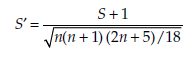
tends towards a standard normal distribution. S’ may then be used instead, in association with the decision rules of the standard normal distribution for rejecting or not rejecting the null hypothesis.

2.5. Comparing two variables X and Y measured from two matched samples A and B: Spearman rank correlation test

Research question Are the two variables X and Y, measured for two matched samples A and B, independent?

Application conditions

• The two samples are random and of the same size, n.
• The observations in each of the samples are independent.
• The variables X and Y are at least ordinal.

Hypotheses

Null hypothesis, H₀: X and Y are independent, alternative hypothesis, H₁: X and Y are dependent.

Statistic

The two variables (X, Y) observed in a sample of size n give n pairs of obser­vations (X₁, Y₁), (X₂, Y₂) … (X_n, Y_n). The values of X_i and Y_j can be classed sep­arately in ascending order. Each of the values X_i and Y_j is then attributed a rank
between 1 and n. Let R(X_t) be the rank of the value X_i, R(Y_t) the rank of the value Y and di = R(X) – R(Y).

The Spearman rank correlation coefficient is:

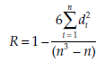
Interpreting the test The Spearman rank correlation coefficient R can be eval­uated in the same way as a classical correlation coefficient (see Sections 4.1 through 4.3 in main Section 2).

2.6. Comparing classifications

Research question Are k classifications of n elements identical?

This type of test can be useful, for instance, when comparing classifications made by k different experts, or according to k different criteria or procedures.

Application conditions

• A set of n elements E₁, E₂, …, E_n has been classified by k different procedures

Hypotheses

Null hypothesis, H₀: the k classifications are identical, alternative hypothesis, H₁: At least one of the k classifications is different from the others

Statistic

The statistic calculated is:

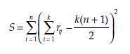
where r_ij is the rank attributed to the element E_i by the procedure j (expert opin­ion, criteria, method …).

The statistic X is compared to critical values X_a available in a table.

Interpreting the test The decision rule is the following:

H₀ will be rejected if S > X_a.

Source: Thietart Raymond-Alain et al. (2001), Doing Management Research: A Comprehensive Guide, SAGE Publications Ltd; 1 edition.