In Chapter 4, Section 4.5 on risk analysis mentioned making most likely (or normal), optimistic, and pessimistic cost estimates for project tasks. Such estimates were shown in Table 4-6, and we promised to illustrate how to use these and similar estimates of task duration to determine the likelihood that a project can be completed by some predetermined time or cost. It is now time to keep that promise.
1. Calculating Probabilistic Activity Times
First, it is necessary to define what is meant by the terms “pessimistic,” “optimistic,” and “most likely” (or “normal”). Assume that all possible durations (or all possible costs) for some task can be represented by a statistical distribution as shown in Figure 5-13. The individual or group making the estimates is asked for a task duration, a, such that the actual duration of the task will be a or lower approximately 3 times out of 1,000 times. Thus a is an optimistic estimate. The pessimistic estimate, b, is an estimated duration for the same task such that the actual finish time will be b or greater approximately 3 times out of 1,000 times. (These estimates are often referred to as the “almost never level.”) The most likely or normal duration is m, which is the mode of the distribution shown in Figure 5-13.
The mean of this distribution, also referred to as the “expected time,” TE, can easily be found in the following way:[1]
TE = (a + 4m + b)/6
For the statisticians among our readers, this calculation gives an approximation of the mean of a beta distribution. The beta distribution is used because it is far more flexible than the more common normal distribution and because it more accurately reflects actual time and cost outcomes. (For the derivation of the approximation, see Kamburowski, 1997; Keefer and Verdini, 1993).[2] The calculation itself is merely a weighted average of the three-time estimates, a, m, and b using weights of 1-4-1, respectively. (For those favoring the triangular distribution, its true mean is (a + m + b)/3 which is another weighted average but with equal weights for the three estimates.)
We can also approximate the standard deviation, o, of the beta distribution as

In this case, the “6” is not a weighted average but rather an assumption that the range of the distribution covers six standard deviations (6a). It follows that the variance of this distribution is estimated as
![]()
The assumption that the range of the distribution, b — a, covers six standard deviations is important. It assumes that the estimator actually attempted to judge a and b so that 99.7 percent of all cases were greater than a and less than b; that is, approximately 3 out of 1,000 cases lay outside of these estimates. We have never met a PM who was comfortable with such extreme levels of likelihood. 99.7 percent translates to “almost never outside the range,” (three standard deviations) leading to estimates of a and b that are so small and large, respectively, as to be nearly useless.
But estimators are not so uncomfortable making estimates at the 95 (or 90) percent levels where a is estimated so that 5 (or 10) percent of all cases are less than a, and 5 (or 10) percent are greater than b. These estimates are within the range of everyday experience. These levels, however, do not cover 6a, so using the above formula for finding the standard deviation will result in a significant underestimation of the uncertainty associated with activity durations and cost estimates. Correcting for such errors is simple. If a and b estimates are made at the 95 percent level, the following should be used to find a (and squared to find the variance):
![]()
If estimates of a and b are made at the 90 percent level
![]()
2. The Probabilistic Network, an Example
Table 5-4 shows a set of tasks, their predecessors, and optimistic, most likely, and pessimistic durations for each activity, plus the expected time and activity duration variance. (If the project had been more realistic, that is, much larger, we would have used an Excel® spreadsheet to handle all the calculations.)
The expected time for each activity was calculated by using the previously noted weighted average of the three time estimates. (The fractional remainders for these calculations are left in sixths for convenience because each TE will be added to others.) For example, to find TE for activity a, we have
Te = (a + 4m + b) / 6
=(8+4(10)+16)/6
= 64/6
= 10.4 days
The variance for a is also easily found as


(The traditional ((b — a)/6)2 was used to calculate the variance, solely because it is traditional. A problem at the end of this chapter will ask the reader to recalculate the variance assuming 95 and 90 percent estimations, thereby repeating some of the calculations shown in this section.)
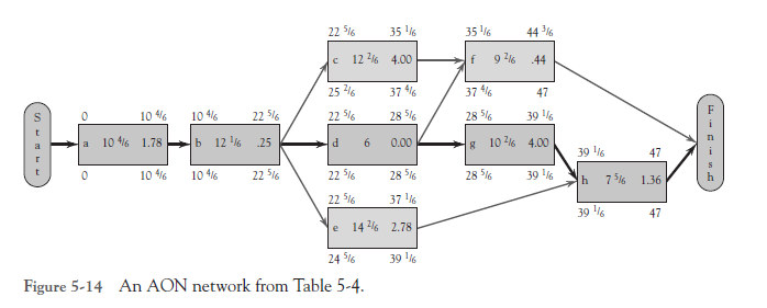
The network associated with the data in Table 5-4 appears in Figure 5-14. Note that the entries inside the nodes are the activity identifier, TE, and variance, in that order. Some activities are known with certainty (i.e., a = m = b), as in task d that takes 6 days in this example. (A real-world example of such an activity would be a 60-day toxicity test of a new drug. In that case, a = m = b = 60 days, not more and not less.) Once in a great while the test may get fouled up and the estimate will be wrong, but our drug manufacturing friends tell us this is quite rare. In some cases, the optimistic and most likely times are the same, a = m. We might, for instance, allow a specific time for paint to dry, a time that is usually sufficient, but may not be if the weather is very humid. Occasionally, the most likely and the pessimistic times may be the same, m = b, as in f. Sometimes the range may be symmetric, (m — a) = (b — m), but more often it is not. Some activities have little uncertainty in duration, which is to say, low variance. Some have high uncertainty, high variance.
The expected time for each activity can be used to find the path with the longest expected time. A forward pass is made, and the “critical path” is found to be a-b-d-g-h. The critical time is 47 days. Because the mean time (TE) is used for all activities, there is a 50-50 probability of completing the project in 47 days or less—and also, 47 days or more. Activity slack is calculated by using a backward pass, exactly as we did in the previous section.
There are several problems with conducting the risk analysis in the way that we are demonstrating. For example, given the uncertainty in path durations, we cannot be sure that a-b-d-g-h is actually the critical path. One of the other paths, a-b-c-f, for example, may turn out to be longer when the project is actually carried out. Remember that a, m, and b are estimates, and remember also that the durations are ranges, not point estimates. We refer to a-b-d-g-h as the critical path solely because it is customary to call the path with the longest expected time the “critical path.” Again, only after the fact do we know which path was actually the critical path. The managerial implication of this caveat is that the PM must carefully manage all paths that have a reasonable chance of being the actual critical path. It is also well to remember that in reality all projects are characterized by uncertainty. Sometimes, with routine maintenance projects, for example, activity variances are quite small, but they are rarely zero.

There are also problems with conducting the same type analysis by use of simulation. We will delay discussions of the assumptions behind these methods and a comparison of the pros and cons of such analyses until we have completed descriptions of both methods. In the meantime, it is helpful to bear in mind that the analysis started in Table 5-4, and continued in Table 5-5, and the simulation methods we then discuss are simply two different methods of accomplishing essentially the same thing.
3. Once More the Easy Way
Just as it did for the deterministic sample network, MSP can easily handle the probabilistic network, though as we will see, it does not do some of the calculations that we demonstrate. Those can be done easily enough in Excel®. The stochastic (a fancy synonym for “probabilistic,” from the Greek word for “conjectural” and pronounced “sta kas’ tic” or “sto kas’ tic”) network used for the preceding discussion is shown as a product of MSP. Table 5-4 becomes MSP Table 5-5, and Figure 5-14 becomes MSP Figure 5-15.
While Figure 5-14 shows the total elapsed time from Day 0 to Day 47 as one proceeds from left to right, the MSP equivalent, Figure 5-15, shows time as start and finish calendar dates. The project starts on February 4 and is completed on April 10. That is a total elapsed calendar time of 67 days. The time appears significantly different from the 47 days that we determined above as being the expected time for the project. The difference is caused by the fact that MSP assumes (defaults to) a 5-day workweek. If you count out the work days on a calendar, you may find that the project seems to take 48 or even 49 days, not 47. That anomaly results from the fact that MSP operates on a real-world calendar. It remembers that February has a national holiday, President’s Day. It also remembers that February has 29 days on leap years, and it was on a leap year that we created this example. (It is not difficult to change the workweek assumption or to add or delete holidays.) Not counting Saturdays, Sundays, holidays, and remembering the leap year, the project has an expected duration of 47 days, as we thought it should.

4. The Probability of Completing the Project on Time
Let us now return to our sample problem of Table 5-4 and Figure 5-14. Recall that the project has an expected critical time of 47 days (i.e., path a-b-d-g-h). How would you respond if your boss said, “The client just called and wants to know if we can deliver the project on April 30, 51 working days from today. I’ve checked, and we can start tomorrow morning.”
You know that path a-b-d-g-h has an expected duration of 47 days, but if you promise delivery in 47 days there is a 50 percent chance that this path will be late, not to mention the possibility that one of the other three paths will take longer than 47 days to complete. That seems to you to be too risky. Tomorrow morning will be 50 working days before April 30, so you wonder: What is the probability that the project will be completed in 50 days or less?
This question can be answered with the information available concerning the level of uncertainty for the various project activities. First, there is an assumption that should be noted. The individual variances of the activities in a series of activities (such as a path through a network) may be summed to find the variance of the set of activities on the path itself, if the various activities in the set are statistically independent. In effect, statistical independence means the following in this example: If a is a predecessor of b, and if a is early or late, it will not affect the duration of b. Note what this does not say. It does not say that the date when b is completed will not be affected. If a is late, b is also likely to be late, but the time required to accomplish b, its duration, will not be affected. This may be a subtle distinction, but it is important because the condition of statistical independence is often met by project activities, and this allows us to answer the boss’s question seriously.
There are times when the assumption of statistical independence is not met. For example, assume two activities require some software code to be written. If during the project the code writer originally assigned to the project becomes unavailable and a less experienced code writer is assigned to the tasks, the times to complete these two tasks are clearly not independent of one another. If the lack of experience increases the task time and/or variance of one task, it is likely to impact other tasks in the same fashion. In this case, one should deal with the problem by reestimating the duration of both tasks. In general, this should be done anytime the resources supplied to a project are different from those presumed when the duration of project activities was originally estimated.
To complete a project by a specified time requires that all the paths in the project’s network be completed by the specified time. Therefore, determining the probability that a project is completed by a specified time requires calculating the probability that all paths are finished by the specified time. Then based on our assumption that the paths are independent of one another, we can calculate the probability that the entire project is completed within the specified time by multiplying these probabilities together. Again, recall from basic statistics that the probability of multiple independent events all occurring is equal to the product of each event’s individual probability of occurrence.
To begin, let’s evaluate the probability that path a-b-d-g-h, which is apparently the critical path, will be completed on or before 50 days after the project is started. We can find the probability by finding z in the following equation:
![]()
where:

The exact nature of z will become clear shortly. Using the problem at hand, p = 47 days, D = 50 days, and 1.78 + .25 .00 + 4.00 + 1.36 7.39. (The square root of 7.39 = 2.719.) Using these numbers, we find
z = (50-47)/2.719 = 1.10
Because the square root of the variance of a statistical distribution equals the standard deviation of that distribution, z is the number of standard deviations separating D and p. The distribution in question is the distribution of the time required to complete the path a-b-d-g-h. Consider all possible combinations of the activity times of the tasks on this path. This would include all possibilities from a combination of all optimistic times to a combination of all pessimistic times and everything in between. And even this does not include the highest and lowest project duration outcomes because the estimates do not cover 100 percent of all possible activity times; they cover only 99 + percent. We can illustrate the frequency distribution of the critical path completion times in Figure 5-16. (The Central Limit theorem allows the use of a normal distribution.)

The calculation of z made above shows the desired date, D, to be approximately 1.1 standard deviations above the expected critical time, p, for the project. If we define the total area under the curve as 1.0 (100 percent of all times), then the area under the curve to the left of 50 days is equivalent to the probability that the path a-b-d-g-h will be completed in 50 days or less.
The table with the cumulative probabilities for the normal distribution on the inside back cover of the book shows the probability associated with a wide range of values of z. For z = 1.10, the probability is .8643 or about 86 percent that this path will be finished on or before Day 50. Again, we remind you that because of uncertainty, other paths may turn out to be critical, possibly delaying the project. Therefore, calculating the probability that the entire project is completed by some specified date requires calculating the probability that all paths that comprise the project are finished by the specified time.
Similar calculations are next done for paths a-b-c-f, a-b-e-h, and a-b-d-f. The probabilities of each of these paths being completed by Day 50 are 98.5 percent, 97.8 percent, and virtually 100 percent, respectively. Based on this, the probability that the entire project is completed by Day 50 is calculated as .864 x .985 x .978 x 1.000 = .832 or 83.2 percent.
A few comments are relevant at this point. First, to simplify the task of calculating the probability that a project is completed by a specified time, for practical purposes it is reasonable to consider only those paths whose expected completion times have a reasonable chance of being greater than the specified time. For example, if the sum of a path’s expected time and 2.33 of its standard deviations is less than the specified time, then the probability of this path taking longer than the specified time is quite small, less than 1 percent (2.06 standard deviations would be less than 2 percent). We simply assume that there is a negligible probability that the path will cause the project to be late. For example, path a-b-d-f’s expected time and standard deviation are 38.2 and 1.57, respectively. Using this rule of thumb, we get 38.2 + (2.33 x 1.57) = 41.9, which is much less than 50. Since there is less than a 1 percent chance this path will take longer than 41.9 days, there is no need to consider the possibility that it will take longer than 50 days.
Second, to calculate the probability that a project will take longer than any specified time, we must first calculate the probability that it will take less than the specified time. Subtracting that probability from 1 gives us the probability that it will take longer than the specified time.
Finally, Excel®’s NORM.DIST function can be used as an alternative to tables of cumulative probabilities for the normal distribution for calculating the probability that a path finishes by a specified time, D. The syntax of this function is as follows:
![]()
To illustrate, the probability that path a-b-d-g-h is completed on or before 50 days can be calculated with Excel® as = NORM.DIST (50, 47,2.719, TRUE).
5. Selecting Risk and Finding D
We can also work this problem backwards. Assume that a client is very important, very demanding, and will be very upset if the project is late. The client has asked when the project output will be available. The client insists on a firm date. How sure do you wish to be about being on time? (Don’t say 100 percent because that implies a time so long that no one will believe you.) Carefully considering the matter, you decide that you want a 95 percent probability of meeting your promised completion date. When should you tell the client to expect delivery?
This is the same problem solved just above, but now D, the desired date, is the unknown while the probability associated with z is preset at .95. Referring to the table with cumulative probabilities for the normal distribution on the inside back cover we can see that for a .95 probability, z will have a value of 1.645. Therefore,

Say, noon of the 52nd day. Note, this result indicates that there is a 95 percent chance of completing path a-b-d-g-h in 51.5 days. Remember that this does not mean that there is a 95 percent chance of completing the entire project in 51.5 days.
We can arrive at the same answer using the Excel® NORM.INV function. The syntax of this function is

In our example, this function would be used as follows:

6. The Case of the Unreasonable Boss
What happens if your boss is unreasonable, a “pointy-hair” type who insists that he wants the project we have been discussing delivered in 45 days instead of the later delivery times we have considered thus far? To find the likelihood that you can deliver, we return to z.
In this case,

Reference to the cumulative probability table displayed on the inside cover of the book reveals that there are no negative zs. This merely indicates that D is less than p. A glance at Figure 5-16 will show this because 45 is to the left of p. To find the probability associated with a negative z, we find the probability of z as if it were a positive number—for z = .74. Because the table with cumulative probabilities on the inside back cover is based on a normal distribution which is symmetric, the negative z will be as far below m as the positive z is above it. Therefore, for a negative number the probability will be 1 minus the probability for the same positive number, p( — z) = 1—p(z).
The probability for z = .74 is .77 and thus the probability of z = —.74 is (1 — .77) = .23. (With Excel®’s NORM.DIST and NORM.INV functions, this transformation is not required.) As the PM—other things being the same—you have between a 1 in 4 and a 1 in 5 chance of completing the project on time, not very good odds. The weasel words “other things being the same” will be removed in the next chapter when we reconsider the problem of the pointy-haired boss.
7. A Potential Problem: Path Mergers
When two or more paths through a network join, even at the end of the network, paths that have little slack and/or high variance may become critical simply by chance. For example, examine path a-b-c-f in Figure 5-14, a path with an expected duration of 44.5 days and a path variance of 6.47 days. What is the chance that this path could be longer than our expected project completion time of 47 days?
As we noted earlier, elementary probability theory (see Appendix ) states that if the probability of event A occurring is P(A) and the probability of event B occurring is P(B), then the probability of both events A and B occurring is P(A) x P(B), assuming the events are independent. Tasks a and b are common to both paths, so we ignore them. Tasks d, g, and h have an expected duration of 24.17 days, and their path has a variance of 5.36. Tasks c and f have an expected duration of 21.67 days, and that path has a 4.44 variance. Because d, g, and h have an expected completion time of 24.17 days, there is .5 chance these activities will take longer than 24.17 days. Therefore, we can ask: What is the probability that the c-f path will exceed 24.17 days? Back to z.

An examination of the cumulative probability table displayed on the inside cover of the book shows that for z equal to 1.18 the probability that the path c-f will be 24.17 days or less is .88. Using Excel® we can write = NORM.DIST (24.17, 21.67, 2.11, TRUE). The probability that both paths will be 24.17 days or less is .5 x .88 = .44.
As we see, the probability of completing the project by 47 days has now dropped from 50 percent to 44 percent. Are there any other paths that may further reduce our expectations of finishing in 47 days? Indeed, path a-b-e-h could also delay the project and, as it happens, reduces the probability further to 38 percent. So we see that probabilities based solely on the apparent critical path may be quite optimistic, depending on the slack and variance of other paths in the project. Hence it is important to examine the network closely to see if any other paths might threaten our estimates of completion. In this case, the original due date was set high enough that these alternative paths are not a problem and the chance that all three will be completed by Day 50, the boss’s original due date, is still well above 80 percent. The reason for introducing some slack for the entire project is now clear. It should also be clear that given a large project with considerable uncertainty and many paths from start to finish, this manner of dealing with risk is lengthy and probably tedious. More important than tedium, at times the assumption of statistical independence of the paths is not met. There is an alternative way to deal with risk, but it is based firmly on the concepts and issues we have just discussed, so they must be understood before tackling the alternative, simulation.
Uncertainty and risk management are introduced. Optimistic, most likely, and pessimistic estimates of task duration are made and expected activity times are calculated as well as the standard deviation and variance of task time distributions. From this data the mean times for all paths are calculated, and the probability of the paths being completed on or before a predetermined date can be found. In addition, the probability of completion can be set in advance and the path delivery date consistent with that probability can be determined. The problem of path mergers is then investigated.
Source: Meredith Jack R., Mantel Jr. Samuel J., Shafer Scott M., Sutton Margaret M. (2017), Project Management in Practice, John Wiley & Sons, Inc. 3th Edition.
8 Jun 2021
8 Jun 2021
8 Jun 2021
8 Jun 2021
8 Jun 2021
8 Jun 2021