Statistical Process Control in Production and Operation Management

Statistical process control (SPC) is the application of statistical techniques to determine whether the output of a process conforms to the product or service design. It aims at achieving good quality during manufacture or service through prevention rather than detection. It is concerned with controlling the process that makes the product because if the process is good then the product will automatically be good.

1. Control Charts

SPC is implemented through control charts that are used to monitor the output of the process and indicate the presence of problems requiring further action. Control charts can be used to monitor processes where output is measured as either variables or attributes. There are two types of control charts: Variable control chart and attribute control chart.

1. Variable control charts: It is one by which it is possible to measures the quality characteristics of a product. The variable control charts are X-BAR chart, R-BAR chart, SIGMA
2. Attribute control chart: It is one in which it is not possible to measures the quality characteristics of a product, e., it is based on visual inspection only like good or bad, success or failure, accepted or rejected. The attribute control charts are p-charts, np-charts, c-charts, u-charts. It requires only a count of observations on characteristics e.g., the number of non­conforming items in a sample.

CHARACTERISTICS OF CONTROL CHARTS

A control chart is a time-ordered diagram to monitor a quality characteristic, consisting of:

1. A nominal value, or centre line, the average of several past samples.
2. Two control limits used to judge whether action is required, an upper control limit (UCL) and a lower control limit (LCL).
3. Data points, each consisting of the average measurement calculated from a sample taken from the process, ordered overtime. By the Central Limit Theorem, regardless of the distribution of the underlying individual measurements, the distribution of the sample means will follow a normal distribution. The control limits are set based on the sampling distribution of the quality measurement.

BENEFITS OF USING CONTROL CHARTS

Benefits of Using Control Charts Following are the benefits of control charts:

1. A control chart indicates when something may be wrong, so that corrective action can be taken.
2. The patterns of the plot on a control chart diagnosis possible cause and hence indicate possible remedial actions.
3. It can estimate the process capability of process.
4. It provides useful information regarding actions to take for quality improvement.

OBJECTIVES OF CONTROL CHARTS

Objectives of Control Charts Following are the objectives of control charts:

1. To secure information to be used in establishing or changing specifications or in determining whether the process can meet specifications or not.
2. To secure information to be used on establishing or changing production procedures.
3. To secure information to be used on establishing or changing inspection procedures or acceptance procedures or both.
4. To provide a basis for current decision during production.
5. To provide a basis for current decisions on acceptance for rejection of manufacturing or purchased product.
6. To familiarize personnel with the use of control chart.

CONTROL CHARTS FOR VARIABLES

As the name indicates, these charts will use variable data of a process. X chart given an idea of the central tendency of the observations. These charts will reveal the variations between sample observations. R chart gives an idea about the spread (dispersion) of the observations. This chart shows the variations within the samples.

X-Chart and R-Chart: The formulas used to establish various control limits are as follows:

(а)   Standard Deviation of the Process, a, Unknown

R-Chart: To calculate the range of the data, subtract the smallest from the largest measurement in the sample.

The control limits are:     

where

R = average of several past R values and is the central line of the control chart, and

D₃, D₄ = constants that provide three standard deviation (three-sigma) limits for a given sample size

X-Chart: The control limits are:

(b)   Standard Deviation of the Process, a, Known

Control charts for variables (with the standard deviation of the process, a, known) monitor the mean, X, of the process distribution.

The control limits are:

where

x = centre line of the chart and the average of several past sample means, Z is the standard normal deviate (number of standard deviations from the average),

 and is the standard deviation of the distribution of sample means, and n is the sample size

Procedures to construct X-chart and R-chart 1.

1. Identify the process to be controlled.
2. Select the variable of interest.
3. Decide a suitable sample size (n) and number of samples to be collected (k).
4. Collect the specified number of samples over a given time interval.
5. Find the measurement of interest for each piece within the sample.
6. Obtain mean (X) of each sample.
7. Establish control limits for X and R-charts.

CONTROL CHARTS FOR ATTRIBUTES

P-charts and C-charts are charts will used for attributes. This chart shows the quality characteristics rather than measurements.

P-Chart

A p-chart is a commonly used control chart for attributes, whereby the quality characteristic is counted, rather than measured, and the entire item or service can be declared good or defective.

The standard deviation of the proportion defective, p, is:

 where

n = sample size,

and p = average of several past p values and central line on the chart.

Using the normal approximation to the binomial distribution, which is the actual distribution of p

 

where z is the normal deviate (number of standard deviations from the average).

ILLUSTRATIONS ON X BAR CHART AND R BAR CHART

1. Standard Deviation of the Process, L, Unknown

ILLUSTRATION 1: Several samples of size n = 8 have been taken from today’s production of fence posts. The average post    was 3 yards in length and the average sample range was 0.015 yard. Find the 99.73% upper and lower control limits.

SOLUTION:

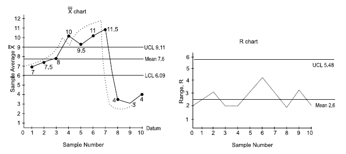
ILLUSTRATION 2 (Problem on X and R Chart): The results of inspection of 10 samples with its average and range are tabulated in the following table. Compute the control limit for the X and R-chart and draw the control chart for the data.

SOLUTION:

Therefore,

For X chart

The values of various factors (like A2, D4 and D3) based on normal distribution can be found from the following table:

A2 = 0.58, D3 = 0 and D4 = 2.11

Thus, for X chart

UCL = 7.6 + (0.58 × 2.6)

= 7.6 + 1.51 = 9.11
LCL = 7.6 – (0.58 × 2.6) = 6.09

For R chart

These control limits are marked on the graph paper on either side of the mean value (line). X and R values are plotted on the graph and jointed, thus resulting the control chart.

From the X chart, it appears that the process became completely out of control for 4th sample over labels.

2. Standard Deviation of the Process, σ, known

ILLUSTRATION 3: Twenty-five engine mounts are sampled each day and found to have an average width of 2 inches, with a standard deviation of 0.1 inche. What are the control limits that include 99.73% of the sample means (z = 3)?

SOLUTION:

ILLUSTRATION 4 (Problem on p-Chart): The following are the inspection results of 10 lots, each lot being 300 items. Number defectives in each lot is 25, 30, 35, 40, 45, 35, 40, 30, 20 and 50. Calculate the average fraction defective and three sigma limit for P-chart and state whether the process is in control.

SOLUTION:

Upper Control Limit,

Conclusion: All the samples are within the control limit and we can say process is under control.

TYPES OF SAMPLING ERRORS

There are two types of errors. They are type-I and type-II that can occur when making inferences from control chart.

Type-I: Error or a-error or Level of Significance

Reject the hypothesis when it is true.

This results from inferring that a process is out of control when it is actually in control. The probability of type-I error is denoted by a, suppose a process is in control. If a point on the control chart falls outside the control limits, we assume that, the process is out of control. However, since the control limits are a finite distance (3a) from the mean. There is a small chance about 0.0026 of a sample falling outside the control limits. In such instances, inferring the process is out of control is wrong conclusion.

The control limits could be placed sufficiently far apart say 4 or 5a stand deviations on each side of the central lines to reduce the probability of type-I error.

Type-II: Error or 0-error

Accept the hypothesis when it is false.

This results from inferring that a process is in control when it is really out of control. If no observations for outside the control limits we conclude that the process is in control while in reality it is out control. For example, the process mean has changed.

The process could out of control because process variability has changed (due to presence of new operator). As the control limits are placed further apart the probability of type-II error increases. To reduce the probability of type-II error it tends to have the control limits placed closer to each other. This increases the probability of type-I error. Thus, the two types of errors are inversely related to each other as the control limits change. Increasing the sample size can reduce both a and p.

2. Acceptance Sampling

The objective of acceptance sampling is to take decision whether to accept or reject a lot based on sample’s characteristics. The lot may be incoming raw materials or finished parts.

An accurate method to check the quality of lots is to do 100% inspection. But, 100% inspection will have the following limitations:

• The cost of inspection is high.
• Destructive methods of testing will result in 100% spoilage of the parts.
• Time taken for inspection will be too long.
• When the population is large or infinite, it would be impossible or impracticable to inspect each unit.

Hence, acceptance-sampling procedure has lot of scope in practical application. Acceptance sampling can be used for attributes as well as variables.

Acceptance sampling deals with accept or reject situation of the incoming raw materials and finished goods. Let the size of the incoming lot be N and the size of the sample drawn be n. The probability of getting a given number of defective goods parts out a sample consisting of n pieces will follow binomial distribution. If the lot size is infinite or very large, such that when a sample is drawn from it and not replaced, then the usage of binomial distribution is justified. Otherwise, we will have to use hyper-geometric distribution.

Specifications of a single sampling plan will contain a sample size (n) and an acceptance number C. As an example, if we assume the sample size as 50 and the acceptance number as 3, the interpretation of the plan is explained as follows: Select a sample of size 50 from a lot and obtain the number of defective pieces in the sample. If the number of defective pieces is less than or equal to 3, then accept the whole lot from which the sample is drawn. Otherwise, reject the whole lot. This is called single sampling plan. There are several variations of this plan.

In this process, one will commit two types of errors, viz, type-I error and type-II error. If the lot is really good, but based on the sample information, it is rejected, then the supplier/ producer will be penalized. This is called producer’s risk or type-I error. The notation for this error is a. On the other hand, if the lot is really bad, but it is accepted based on the sample information, then the customer will be at loss. This is called consumer’s risk or type-II error. The notation for this error is p. So, both parties should jointly decide about the levels of producer’s risk (a) and consumer’s risk (P) based on mutual agreement.

OPERATING CHARACTERISTIC CURVE (O.C. CURVE)

The concepts of the two types of risk are well explained using an operating characteristic curve. This curve will provide a basis for selecting alternate sample plans. For a given value of sample size (n), acceptance number (C), the O.C. curve is shown in Fig. 6.8.

In Fig. 6.9, per cent defective is shown on x-axis. The probability of accepting the lot for given per cent defective is shown on y-axis. The value for per cent defective indicates the quality level of the lot inspected. AQL means acceptable quality level and LTPD indicates lot tolerance per cent defectives. These represent quality levels of the lot submitted for inspection. If the quality level of the lot inspected is at AQL or less than AQL, then the customers are satisfied with the quality of the lot. The corresponding probability of acceptance is called 1 – a. On the other hand, if the quality level is more than or equal to LTPD, the quality of the lot is considered to be inferior from consumer’s viewpoint. The corresponding probability of acceptance of the lot is called p. The quality levelling between AQL and LTPD is called indifferent zone.

So, we require a, p, AQL and LTPD to design a sample plan. Based on these, one can determine n and C for the implementation purpose of the plan.

Fig. 6.10 shows a various O.C. curves for different combinations of n and C.

SINGLE SAMPLING PLAN

The design of single sampling plan with a specified producer’s risk and consumer’s risk is demonstrated in this section. The required data for designing such plan are as follows:

• Producer’s Risk (a)
• Consumer’s Risk (b)
• Acceptable Quality Level (AQL)
• Lot Tolerance Per cent Defectives (LPTD)

The objective of this design is to find out the values for the sample size (n) and acceptance number (C). The values for n and C are to be selected such that the O.C. curve passes through the following two coordinates:

• Coordinate with respect to the given a and AQL.
• Coordinate with respect to the given P and LTPD.

But, the values of n and C should be integers. So, it will be very difficult to find n and C exactly for the given parameters of the design. Hence, we will have to look for approximate integer values for n and C such that the O.C. curve more or less passes through the above two coordinates.

Source: KumarAnil, Suresh N. (2009), Production and operations management, New Age International Pvt Ltd; 2nd Ed. edition.