The Common Metrics in Meta-Analysis: Correlation, Standardized Mean Difference, and Odds Ratio

1. Significance Tests Are Not Effect Sizes

Before describing what effect sizes are, I describe what they are not. Effect sizes are not significance tests, and significance tests are not effect sizes. Although you can usually derive effect sizes from the results of significance tests, and the magnitude of the effect size influences the likelihood of find­ing statistically significant results (i.e., statistical power), it is important to distinguish between indices of effect size and statistical significance.

Imagine that a researcher, Dr. A, wishes to investigate whether two groups (male versus female, two treatment groups, etc.) differ on a particular variable X. So she collects data from five individuals in each group (N = 10). She finds that Group 1 members have scores of 4, 4, 3, 2, and 2, for a mean of 3.0 and (population estimated) standard deviation of 1.0, whereas Group 2 members have scores of 6, 6, 5, 4, and 4, for a mean of 5.0 and standard devia­tion of 1.0. Dr. A performs a t-test and finds that t(8) = 3.16, p = .013. Finding that Group 2 was significantly higher than Group 1 (according to traditional criteria of a = .05), she publishes the results.

Further imagine that Dr. B reads this report and is skeptical of the results. He decides to replicate this study, but collects data from only three individu­als in each group (N = 6). He finds that individuals in Group 1 had scores of 4, 3, and 2, for a mean of 3.0 and standard deviation of 1.0, whereas Group 2 members had scores of 6, 5, and 4, for a mean of 5.0 and standard deviation of 1.0. His comparison of these groups results in £(4) = 2.45, p = .071. Dr. B concludes that the two groups do not differ significantly and therefore that the findings of Dr. A have failed to replicate.

Now we have a controversy on our hands. Graduate student C decides that she will resolve this controversy through a definitive study involving 10 individuals in each group (N = 20). She finds that individuals in Group 1 had scores of 4, 4, 4, 4, 3, 3, 2, 2, 2, and 2, for a mean of 3.0 and standard devia­tion of 1.0, whereas individuals in Group 2 had scores of 6, 6, 6, 6, 5, 5, 4, 4, 4, and 4, for a mean of 5.0 and a standard deviation of 1.0. Her inferential test is highly significant, £(18) = 4.74, p = .00016. She concludes that not only do the groups differ, but also the difference is more pronounced than previously thought!

This example illustrates the limits of relying on the Null Hypothesis Significance Testing Framework in comparing results across studies. In each of the three hypothetical studies, individuals in Group 1 had a mean score of 3.0 and a standard deviation of 1.0, whereas individuals in Group 2 had a mean score of 5.0 and a standard deviation of 1.0. The hypothetical research­ers’ focus on significance tests led them to inappropriate conclusions: Dr. B’s conclusion of a failure to replicate is inaccurate (because it does not consider the inadequacy of statistical power in the study), as is Student C’s conclusion of a more pronounced difference (which mistakenly interprets a low p value as informing the magnitude of an effect). A focus on effect sizes would have alleviated the confusion that arose from a reliance only on statistical signifi­cance and, in fact, would have shown that these three studies provided per­fectly replicating results. Moreover, if the researchers had considered effect sizes, they could have moved beyond the question of whether the two groups differ to consider also the question of how much the two groups differ. These limitations of relying exclusively on significance tests have been the subject of much discussion (see, e.g., Cohen, 1994; Fan, 2001; Frick, 1996; Harlow, Mulaik, & Steiger, 1997; Meehl, 1978; Wilkinson & the Task Force on Statis­tical Significance, 1999), yet this practice unfortunately persists.

For the purposes of most meta-analyses, I find it useful to define an effect size as an index of the direction and magnitude of association between two vari- ables.¹ As I describe in more detail later in this chapter, this definition includes traditional measures of correlation between two variables, differences between two groups, and contingencies between two dichotomies. When conducting a meta-analysis, it is critical that effect sizes be comparable across studies. In other words, a useful effect size for meta-analysis is one to which results from various studies can be transformed and therefore combined and compared. In this chapter I describe ways that you can compute the correlation (r), standard­ized mean difference (g), or odds ratio (o) from a variety of information com­monly reported in primary studies; this is another reason that these indexes are useful in summarizing or comparing findings across studies.

A second criterion for an effect size index to be useful in meta-analysis is that it must be possible to compute or approximate its standard error. Although I describe this importance more fully in Chapter 8, I should say a few words about it here. Standard errors describe the imprecision of a sam­ple-based estimate of a population effect size; formally, the standard error represents the typical magnitude of differences of sample effect sizes around a population effect size if you were to draw multiple samples (of a certain size N) from the population. It is important to be able to compute standard errors of effect sizes because you generally want to give more weight to studies that provide precise estimates of effect sizes (i.e., have small standard errors) than to studies that provide less precise estimates (i.e., have large standard errors). Chapter 8 of this book provides further description of this idea.

Having made clear the difference between statistical significance and effect size, I next describe three indices of effect size that are commonly used in meta-analyses.

2. Pearson Correlation

The Pearson correlation, commonly represented as r, represents the asso­ciation between two continuous variables (with variants existing for other forms, such as rpb when one variable is dichotomous and the other is continu­ous, φ when both are dichotomous). The formula for computing r (the sample estimate of the population correlation, p) within a primary data set is:

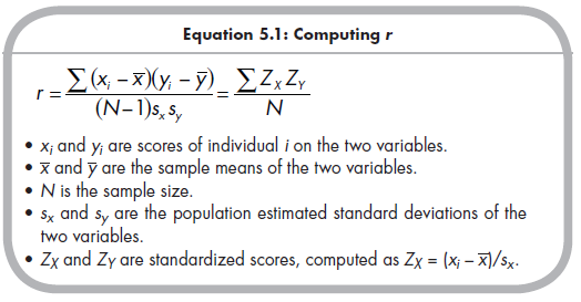
The conceptual meaning of positive correlations is that individuals who score high on X (relative to the sample mean on X) also tend to score high on Y (relative to the sample mean on Y), whereas individuals who score low on X also tend to score low on Y. The conceptual meaning of negative correlations is that individuals who score high on one variable tend to score low on the other variable. The rightmost portion of Equation 5.1 provides an alternative representation that illustrates this conceptual meaning. Here, Z scores (stan­dardized scores) represent high values as positive and low values as negative, so a preponderance of high scores with high scores (product of two positive) and low scores with low scores (product of two negative) yields a positive average cross product, whereas high scores with low scores (product of posi­tive and negative) yield a negative average cross product.

You are probably already familiar with the correlation coefficient, but per­haps are not aware that it is an index of effect size. One interpretation of the cor­relation coefficient is in describing the proportion of variance shared between two variables with r². For instance, a correlation between two variables of r = .50 implies that 25% (i.e., .50²) of the variance in these two variables overlaps. It can also be kept in mind that the correlation is standardized, such that cor­relations can range from 0 to ± 1. Given the widespread use of the correlation coefficient, many researchers have an intuitive interpretation of the magnitude of correlations that constitute small or large effect sizes. To aid this interpreta­tion, you can consider Cohen’s (1969) suggestions of r = ± .10 representing small effect sizes, r = ± .30 representing medium effect sizes, and r = ± .50 representing large effect sizes. However, you should bear in mind that the typical magnitudes of correlations found likely differ across areas of study, and one should not be dogmatic in applying these guidelines to all research domains.

In conclusion, Pearson’s r represents a useful, readily interpretable index of effect size for associations between two continuous variables. In many meta-analyses, however, r is transformed before effect sizes are combined or compared across studies (for contrasting views see Hall & Brannick, 2002; Hunter & Schmidt, 2004; Schmidt, Hunter, & Raju, 1988). Fisher’s transfor­mation of r, denoted as Z_r, is commonly used and shown in Equation 5.2.

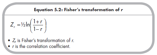
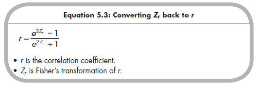
The reason that r is often transformed to Z_r in meta-analyses is because the distribution of sample r’s around a given population p is skewed (except in sample sizes larger than those commonly seen in the social sciences), whereas a sample of Z_rs around a population Z_r is symmetric (for further details see Hedges & Olkin, 1985, pp. 226-228; Schulze, 2004, pp. 21-28).² This sym­metry is desirable when combining and comparing effect sizes across studies. However, Z_r is less readily interpretable than r both because it is not bounded (i.e., it can have values greater than ±1.0) and simply because it is unfamil­iar to many readers. Typical practice is to compute r for each study, convert these to Z_r for meta-analytic combination and comparison, and then convert results of the meta-analysis (e.g., mean effect size) back to r for reporting. Equation 5.3 converts Z_r back to r.

Although I defer further description until Chapter 8, I provide the equa­tion for the standard error here, as you should enter these into your meta­analytic database during the coding process. The standard error of Z_r is shown in Equation 5.4.

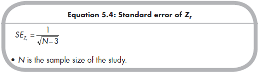
This equation reveals an obvious relation inherent to all standard errors: As sample size (N) increases, the denominator of Equation 5.4 increases and so the standard error decreases. A desirable feature of Z_r is that its standard error depends only on sample size (as I describe later, standard errors of some effects also depend on the effect sizes themselves).

3. Standardized Mean Difference

The family of indices of standardized mean difference represents the mag­nitude of difference between the means of two groups as a function of the groups’ standard deviations. Therefore, you can consider these effect sizes to index the association between a dichotomous group variable and a continu­ous variable.

There are three commonly used indices of standardized mean difference (Grissom & Kim, 2005; Rosenthal, 1994).³ These are Hedges’s g, Cohen’s d, and Glass’s index (which I denote as gGla_ss),⁴ defined by Equations 5.5, 5.6, and 5.7, respectively:

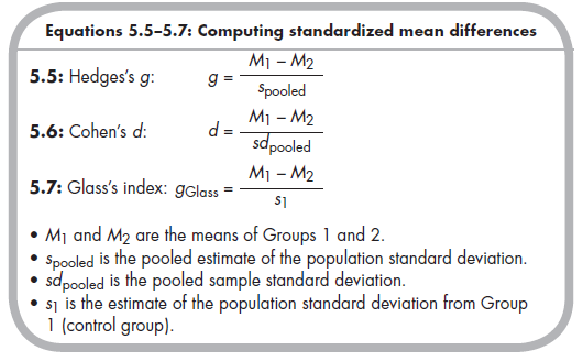
These three equations are identical in consisting of a raw (unstandard­ized) difference of means as their numerators. The difference among them is in the standard deviations comprising the denominators (i.e., the standardiza­tion of the mean difference). The equation (5.5) for Hedges’s g uses the pooled estimates⁵ of the population standard deviations of each group, which is the familiar . The equation (5.6) for Cohen’s d is similar but instead uses the pooled sample standard deviations,  sample standard deviation is a biased estimation of the population standard deviation, with the underestimation greater in smaller than larger samples. However, with even modestly large sample sizes, g and d will be virtually identical, so the two indices are not always distinguished.⁶ Often, people describe both indices as Cohen’s d, although it is preferable to use precise terminology in your own writing.⁷

The third index of standardized mean difference is gGla_ss (sometimes denoted with Δ or g’), shown in Equation 5.7. Here the denominator consists of the (population estimate of the) standard deviation from one group. This index is often described in the context of therapy trials, in which the control group is said to provide a better index of standard deviation than the therapy group (for which the variability may have also changed in addition to the mean). One drawback to using gGla_ss in meta-analysis is that it is necessary for the primary studies to report these standard deviations for each group; you can use results of significance tests (e.g., £-test values) to compute g or d, but not gGlass. Reliance on only one group to estimate the standard deviation is also less precise if the standard deviations of the two populations are equal (i.e., homoscedastic; see Hedges & Olkin, 1985). For these reasons, meta­analysts less commonly rely on g_Glass relative to g or d. On the other hand, if the population standard deviations of the groups being compared differ (i.e., heteroscedasticity), then g or d may not be meaningful indexes of effect size, and computing these indexes from inferential statistics reported (e.g., £-tests, F-ratios) can be inappropriate. In these cases, reliance on gGla_ss is likely more appropriate if adequate data are reported in most studies (i.e., means and standard deviations from both groups).⁸ If it is plausible that heteroscedastic­ity might exist, you may wish to compare the standard deviations (see Shaf­fer, 1992) of two groups among the studies that report these data and then base the decision to use gGla_ss versus g or d depending on whether or not (respectively) the groups have different variances.

Examining Equations 5.5—5.7 leads to two observations regarding the standardized mean difference as an effect size. First, these can be either posi­tive or negative depending on whether the mean of Group 1 or 2 is higher. This is a desirable quality when your meta-analysis includes studies with potentially conflicting directions of effects. You need to be consistent in considering a par­-ticular group (e.g., treatment vs. control, males vs. females) as Group 1 versus 2 across studies. Second, these standardized mean differences can take on any values. In other words, they are not bounded by ±1.00 like the correlation coefficient r. Like r, a value of 0 implies no effect, but standardized mean dif­ferences can also have values greater than 1. For example, in the hypothetical example of three researchers given earlier in this chapter, all three researchers would have found g = (3 – 5)/1 = -2.00 if they considered effect sizes.

Although not as commonly used in primary research as r, these stan­dardized mean differences are intuitively interpretable effect sizes. Knowing that the two groups differ by one-tenth, one-half, one, or two standard devia­tions (i.e., g or d = 0.10, 0.50, 1.00, or 2.00) provides readily interpretable information about the magnitude of this group difference.⁹ As with r, Cohen (1969) provided suggestions for interpreting d (which can also be used with g or gGla_ss), with d = 0.20 considered a small effect, d = 0.50 considered a medium effect, and d = 0.80 considered a large effect. Again, it is important to avoid becoming fixated on these guidelines, as they do not apply to all research situations or domains. It is also interesting to note that transforma­tions between r and d (described in Section 5.5) reveal that the guidelines for interpreting each do not directly correspond.

As I did for the standard error of Z_r, I defer further discussion of weight­ing until Chapter 8. However, the formulas for the standard errors of the commonly used standardized mean difference, g, should be presented here:

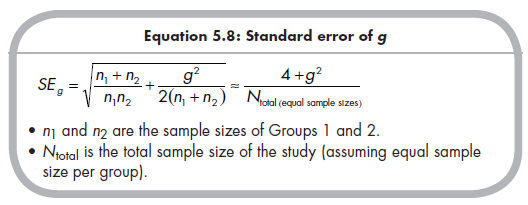
I draw your attention to two aspects of this equation. First, you should use the first equation when sample sizes of the two groups are known; the second part of the equation is a simplified version that can be used if group sizes are unknown, but it is reasonable to assume approximately equal group sizes. Sec­ond, you will notice that the standard errors of estimates of the standardized mean differences are dependent on the effect size estimates themselves (i.e., the effect size appears in the numerators of these equations). In other words, there is greater expected sampling error when the magnitudes (positive or negative) of standardized mean differences are large than when they are small. As dis­cussed later (Chapter 8), this means that primary studies finding larger effect sizes will be weighted relatively less (given the same sample size) than primary studies with smaller effect sizes when results are meta-analytically combined.

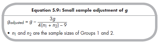
Before ending this discussion of standardized mean difference effect sizes, it is worth considering a correction that you should use when primary study sample sizes are small (e.g., less than 20). Hedges and Olkin (1985) have shown that g is a biased estimate of the population standardized mean differences, with the magnitude of overestimation becoming nontrivial with small sample sizes. Therefore, if your meta-analysis includes studies with small samples, you should apply the following correction of g for small sam­ple size (Hedges & Olkin, 1985, p. 79; Lipsey & Wilson, 2001, p. 49):

4. Odds Ratio

The odds ratio, which I denote as o (OR is also commonly used), is a useful index of effect size of the contingency (i.e., association) between two dichoto­mous variables. Because many readers are likely less familiar with odds ratios than with correlations or standardized mean differences, I first describe why the odds ratio is advantageous as an index of association between two dichot­omous variables.¹⁰

To understand the odds ratio, you must first consider the definition of odds. The odds of an event is defined as the probability of the event (e.g., of scoring affirmative on a dichotomous measure) divided by the probabil­ity of the alternative (e.g., of scoring negative on the measure), which can be expressed as odds = p / (1 – p), where p equals the proportion in the sample (which is an unbiased estimate of population proportion, n) having the characteristic or experiencing the event. For example, if you conceptual­ized children’s aggression as a dichotomous variable of occurring versus not occurring, you could find the proportion of children who are aggressive (p) and estimate the odds of being aggressive by dividing by the proportion of children who are not aggressive (1 – p). Note that you can also compute odds for nominal dichotomies; for example, you could consider biological sex in terms of the odds of being male versus female, or vice versa.

The next challenge is to consider how you can compare probabilities or odds across two groups. This comparison actually indexes an association between two dichotomous variables. For instance, you may wish to know whether boys or girls are more likely to be aggressive, and our answer would indicate whether, and how strongly, sex and aggression are associated. Sev­eral ways of indexing this association have been proposed (see Fleiss, 1994). The simplest way would be to compute the difference between probabilities in two groups, pi – p2 (where pi and p2 represent proportions in each group; in this example, these values would be the proportions of boys and girls who are aggressive). An alternative might be to compute the rate ratio (sometimes called risk ratio), which is equal to the proportion experiencing the event (or otherwise having the characteristics) in one group divided by the pro­portion experiencing it in the other, RR = pi / p2. A problem with both of these indices, however, is that they are highly dependent on the rate of the phenomenon in the study (for details, see Fleiss, 1994). Therefore, studies in which different base rates of the phenomenon are found (e.g., one study finds a high prevalence of children are aggressive, whereas a second finds that very few are aggressive) will yield vastly different differences and risk ratios, even given the same underlying association between the variables. For this reason, these indices are not desirable effect sizes for meta-analysis.

The phi (9) coefficient is another index of association between two dichotomous variables. It is estimated via the following formula (where 9 is the estimated population association):

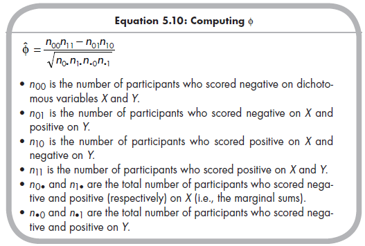
Despite the lack of similarity in appearance between this equation and Equation 5.1, Φ is identical to computing r between the two dichotomous variables, X and Y. In fact, if you are meta-analyzing a set of studies involving associations between two continuous variables in which a small number of studies artificially dichotomize the variables, it is appropriate to compute ^ and interpret this as a correlation (you might also consider correcting for the attenuation of correlation due to artificial dichotomization; see Chapter 6).

However, Φ (like the difference in proportions and rate ratio) also suffers from the limitation that it is influenced by the rates of the variables of inter­est (i.e., the marginal frequencies). Thus studies with different proportions of the dichotomies can yield different effect sizes given the same underlying association (Fleiss, 1994; Haddock, Rindskopf, & Shadish, 1998). To avoid this problem, the odds ratio (o) is preferred when one is interested in associa­tions between two dichotomous variables. The odds ratio in the population is often represented as omega (ω) and is estimated from sample data using the following formula:

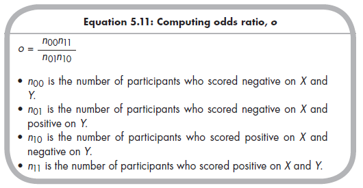
Although this equation is not intuitive, it helps to consider that it repre­sents the ratio of the odds of Y being positive when X is positive [(n11/n1•) / (n10/n1•)] divided by the odds of Y being positive when X is negative [(n01/n0•) / (n00/n0•)], algebraically rearranged.

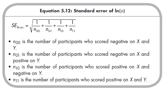
The odds ratio is 1.0 when there is no association between the two dichotomous variables, ranges from 0 to 1 when the association is negative, and ranges from 1 to positive infinity when the association is positive. Given these ranges, the distribution of sample estimates around a population odds ratio is necessarily skewed. Therefore, it is common to use the natural log transformation of the odds ratio when performing meta-analytic combina­-tion or comparison, expressed as ln(o). The standard error of this logged odds ratio is easily computed (whereas computing the standard error of an untransformed odds ratio is more complex; see Fleiss, 1994), using the fol­lowing equation:

Source: Card Noel A. (2015), Applied Meta-Analysis for Social Science Research, The Guilford Press; Annotated edition.