Computing r from Commonly Reported Results

You can compute r from a wide range of results reported in primary studies. In this section, I describe how you can compute this effect size when primary studies report correlations, inferential statistics (i.e., £-tests or F-ratios from group comparisons, x² from analyses of contingency tables), descriptive data, and probability levels of inferential tests. I then describe some more recent approaches to computing r from omnibus test results (e.g., ANOVAs with more than two groups). Table 5.1 summarizes the equations that I describe for computing r, as well as those for computing standardized mean differ­ences (e.g., g) and odds ratios (o).

1. from reported correlations

In the ideal case, primary reports would always report the correlations between variables of interest. This reporting certainly makes our task much easier and reduces the chances of inaccuracies due to computational errors or rounding imprecision. When studies report correlation coefficients, these are often in a tabular form.

TABLE 5.1. Summary of Equations for Computing Effect Sizes from Results of Primary Studies

Although it may be tempting to simply identify this correlation within a table and consider the study coded, it is still important to read the text of the report carefully. This reading may reveal additional information not included in the table that may be of interest, such as other effect sizes or correla­tions separately for subgroups. The text (as well as notes to the tables) may also contain important information regarding the correlation itself, such as whether it was computed for only a subset of the data, was based on a smaller sample size due to pairwise deletion of missing data, or is actually a partial or semipartial correlation due to the control of some other variables.

Although you still need to carefully read studies reporting correlation coefficients, these are much easier to code accurately. Unfortunately, many studies do not report these correlations, so you must turn to other data to code effect sizes. The following can be considered options when studies fail to report actual correlations.

2. From Inferential Statistics

Primary studies will often report results of inferential tests without reporting actual effect sizes (despite recommendations against this practice). This situ­ation can arise in several ways. First, the primary study may simply report the significance test of a correlation coefficient without reporting the coef­ficient itself; most commonly, studies report this significance as a £-test. Sec­ond, the authors of the primary study may have artificially dichotomized one of the variables to form two groups, then compared the groups using an inde­pendent sample £-test or an ANOVA reported as a one degree of freedom (in numerator) F-ratio. Artificially dichotomizing a continuous variable attenu­ates the effect size estimate (see Hunter & Schmidt, 1990; MacCallum et al., 2002), so you might not only compute r as described below but also consider correcting for this dichotomization using the approaches described in Chap­ter 6. A third situation is that the authors of the primary study dichotomized both variables involved in the correlation, then analyzed the data as contin­gency tables and reported a x² statistic with one degree of freedom (a situa­tion in which you would also want to consider corrections for dichotomiza- tion described in Chapter 6).

The following formulas allow us to compute correlations in each of these situations. When primary studies report a £-test value (either for the signifi­cance of the correlation or in comparing two groups), the following equation can be used (Rosenthal, 1991, 1994):

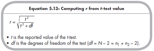
Note that this equation provides either the positive or the negative square root, and it is important to take the value that reflects the direction of the effect in the same way across studies. For instance, if I am interested in the association between relational aggression and rejection, and compute r from a £-test comparing rejection in aggressive versus nonaggressive groups, I need to consider which group has a higher mean when computing the sign of r (positive if the aggressive group is more rejected and negative if the non­aggressive group is more rejected).

Primary studies might alternatively conduct an analysis of variance (ANOVA) between two groups. The resulting inferential statistic is an F-ratio with 1 degree of freedom in the numerator (i.e., Fq/) Because this F-ratio is the same as the square of the parallel £-test, it follows that you can compute a correlation from this value with this equation:

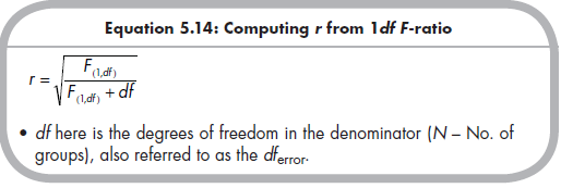
As with the £-test, you must be sure to take either the positive or the negative square root, depending on the direction of mean differences.

Equations 5.13 and 5.14 are for use in converting tests of independent sample £-tests or F-ratios to r. An alternative, albeit less frequent, situation occurs when primary studies report these statistics for repeated-measures (a.k.a. within-subject) comparisons. For instance, a study might report levels of rejection for a sample of children who were aggressive at one time point but not at another. Some recommend against combining independent sample and repeated-measures results in the same meta-analysis (e.g., Lipsey & Wil­son, 2001, state that these should be considered in separate meta-analyses). However, when you believe that the two methodologies address the same effect, you should also explore the moderator variable “type of methodology” (i.e., independent sample versus repeated measures). When computing r, you can use the same formulas (Equations 5.13 and 5.14) for either the inde­pendent sample or repeated-measures £-tests or F-ratios. This is not the case when computing standardize mean differences.

Primary studies might dichotomize both variables of interest and report results as a 2 X 2 contingency tables analysis with a reported x² with 1 degree of freedom. The formula to convert this x² into r is (Rosenthal, 1991, 1994):

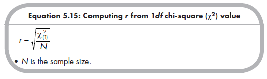
As with computing r from the £-test or F-ratio, it is critical that you take the correct positive or negative square root. To determine which is correct, it is necessary to examine the reported contingency tables: A positive associa­tion is indicated if observed cell frequencies are higher than expected (under the null hypothesis of no association) in the major diagonal (if the contin­gency table is arranged with higher variable values as the lower row and right column), whereas a negative association is indicated if these frequencies are lower than expected. For example, you would consider aggression and rejec­tion to be positively correlated if children who were aggressive and rejected and children who were not aggressive and not rejected occurred more fre­quently than expected.

3. From Descriptive Data

Often primary studies do not report all results that you are interested in as significance tests, but will instead provide descriptive data (often in a table) that can be used to compute r.

Primary studies may present descriptive data (means and standard devi­ations) for one variable based on two groups formed by dichotomizing the other variable (paralleling the case of reported £-tests or F-ratios described above). In this case, it is convenient to compute a standardized mean differ­ence (using Equation 5.5), then transform these into r using Equation 5.26. As with computing r from £-tests and F-ratios, you should consider correcting for the attenuation of effect size due to the artificial dichotomization of the grouping variable (see Chapter 6).

It is also common for primary studies to report results in 2 X 2 contin­gency tables when both variables are dichotomized. In this situation, one can compute ^ using Equation 5.8 and then interpret this ^ as r. You should then correct this correlation for the dichotomization of both variables (see Chapter 6).

4. From Probability Levels of Significance Tests

In some situations, primary studies will not provide any other information other than results of significance tests. The first potential reason for this is simply inadequate reporting of results of a parametric inferential test (i.e., the authors report the statistical significance of a £-test, F-ratio, or x² test of a contingency, but not the value itself). If the exact significance probability is reported for a £-test, two-group ANOVA, or 2 X 2 contingency analysis, one can simply find the corresponding t, F, or x² value at that level of significance and then use Equation 5.13, 5.14, or 5.15 (respectively) to compute r.

A second reason why you might only have probabilities from a signifi­cance test is the primary study’s report of probabilities from nontraditional inferential tests (e.g., nonparametric tests). In these situations in which other methods of computing effect size are unavailable, one can compute effect sizes from these significance tests. To do so, you first identify the exact prob­ability, p, of the significance test and look up the standard normal deviate (i.e., Z) score corresponding to the given two-tailed p that is more extreme than this score (it is important to avoid confusion of this Z-score with the Fisher’s transformation of r, denoted as Z_r, described earlier). For example, if a primary study reported a two-tailed (which is assumed if the study did not specify) p = .032, you would identify the one-tail p as .016 and the corre­sponding Z = 2.14. You can find this corresponding Z-score in tables in many introductory statistics books, although you need to be careful to correctly use these tables (e.g., many tables will list p as the proportion or percentage of the normal distribution between the mean and Z, so it is necessary to look up the Z associated with 0.50 – p or 50 – p, for proportions and percentages, respectively). These tables are also often limited with very small values of p because they frequently do not list these extreme values with enough preci­sion to accurately identify Z. For these reasons, it is often useful to find Z using a computer to identify the inverse of the standard normal cumulative distribution; you can use basic programs such as Microsoft Excel (using the “normsinv” function) to compute exact Z from p.

After computing Z, it is straightforward to compute the corresponding effect size given this value and sample size. The following equation converts Z to r for a given sample size N:

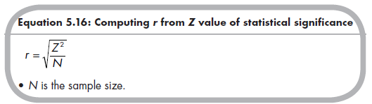
As when computing r from significance tests (t or F), it is important to take either the positive or negative square root from Equation 5.16 to repre­sent the direction of the effect.

In all-too-many primary studies, researchers report a range of probabil­ity but not the exact probability (or associated t or F). For instance, it is not uncommon for primary studies to report that an association or comparison of groups was significant, and then only state that p < .05 (or some other value). In these instances, if the report provides no other information, you cannot compute an exact effect size. You then have two options. The option is to contact the study authors requesting more information, such as the actual effect size, inferential statistic (t or F), or exact significance probability (p). This option is certainly preferable in obtaining accurate effect sizes; unfortu­nately, it is not always possible because authors have retired, left academia, are unwilling to respond to your request, or for any other of numerous rea­sons. In these situations, the second option is to compute the best estimate of effect size given the reported results, which is typically the lower-bound effect size given the upper-bound probability. In other words, if a study reports that p < .05 (let’s say for a sample size of N = 100), you can make the conserva­tive assumption that p = .05 and then compute the associated Z (=1.96) and r (from Equation 5.16, r = √(1.96²/100) = .20). It is important to recognize that this value of r is a lower-bound estimate of the actual effect size found in the primary study. To illustrate, if the true p = .03, r = .22, if p = .01, r = .26, if p = .001, r = .33, and if p = .0001, r = .39, and so on. In other words, if a study only reports that p from a test of significance test is less than some value (e.g., p < .05), you can only conclude that the effect size is greater than some value (e.g., r > .20). Common convention is to be conservative and conduct analyses using this minimum value.

A similar situation of inadequate reporting of data arises when primary studies report only that a particular effect is not statistically significant. In this situation, it is possible to compute a range of possible values of the effect size. To do so, you can compute the Z-score associated with the chosen a (assume a = .05 if not otherwise stated) and then apply Equation 5.15 to determine the maximum magnitude of r that would fail to yield a statisti­cally significant effect given the sample size. You can conclude that the actual effect size of the study was greater than the negative r and less than the positive r. For example, if N = 100, you know that -.20 < r < .20. However, common convention is to take the smallest magnitude effect size—in other words, to assume r = .00.

Taking the minimal effect sizes from primary studies reporting only that the p is less than some value or that an effect size is not significant is clearly not an ideal situation. When this practice is used for a substantial number of studies, the result will be that the mean effect size will be biased toward smaller magnitude (and tests of heterogeneity and moderation also may be biased). The best way to avoid this problem would be to (1) carefully read primary studies for any other information from which effect sizes can be computed and (2) persistently seek further information from authors of the primary studies. If you are still forced to make lower-bound estimates of effect sizes for some studies, it is good practice to (1) report the percentage of included studies for which these lower-bound estimates were made; and (2) conduct a sensitivity analysis by comparing results obtained with these stud­ies versus without them (e.g., conducting two sets of analyses including and excluding these studies, or else evaluating a dichotomous moderator vari­able identifying these studies; one hopes that the impact of these studies is trivial). Alternatively, if many effect sizes (or coded study characteristics) are missing, it might be useful to rely on more recent methods of missing data management (see Pigott, 2009). In Chapters 9 and 10, I describe a structural equation modeling (SEM) representation of meta-analysis that uses sophis­ticated full information maximum likelihood (FIML) methods of handling missing data (Cheung, 2008).

5. From Results of Omnibus Tests

The effect sizes of interest to meta-analysts typically involve associations between two variables. As illustrated earlier, this information is sometimes obtained from two group comparisons on a continuous variable (t-tests or F-ratios with 1 df in numerator). In contrast, some primary studies report results of omnibus tests involving differences among three or more groups (F-ratios with 2 or more numerator dfs). Although exceptions might exist, these omnibus results are generally of little direct use within a meta-analysis. As Rosenthal (1991) poignantly stated, “only rarely is one interested in know­ing . . . that somewhere in the thicket of df there lurk one or more meaningful answers to meaningful questions that we had not the foresight to ask of our data” (p. 13). In other words, you are more often interested in identifying the linear (or other specified form) relations between two variables or the mag­nitudes of differences between two specific groups, more so than whether a number of groups differ in some unspecified way. For example, you might be interested in the linear relation between aggression and rejection from results comparing rejection among children who are aggressive never, some­times, or often, whereas the question of whether there are some differences among these groups (i.e., the omnibus ANOVA) is of less interest. Similarly, you might be interested in a specific comparison of psychosocial intervention versus control conditions from a three-level ANOVA of control, psychoso­cial intervention, and pharmacological intervention conditions. These situa­tions require us to extract meaningful information (i.e., effect sizes) from less meaningful omnibus tests.

Techniques for computing effect sizes from these omnibus tests are described in detail by Rosenthal, Rosnow, and Rubin (2000), and I refer read­ers to this source for complete description. Here, I briefly outline the approach to computing r from descriptive data (i.e., means and standard deviations) or results of one-way ANOVAs with three or more groups. Procedures for man­aging repeated-measures and factorial ANOVAs are described in Rosenthal et al. (2000).

5.1. From Descriptive Statistics

The first situation I consider is when the primary study reports group sizes, means, and standard deviations from three or more groups. The first step in computing the linear association between the independent (i.e., group­ing) and dependent (i.e., outcome) variables is to determine a set of contrast weights for the groups, denoted as Xg for the g groups, such that these con­trast weights sum to zero. The most typical choices of contrast weights are —1, 0, and 1 for three groups; -3, —1, 1, and 3 for four groups; and -2, —1, 0, 1, and 2 for five groups (contrast weights for more groups could be obtained through tables of orthogonal contrast codes, e.g., Cohen, Cohen, West, & Aiken, 2003, p. 215; Rosenthal et al., 2000, p. 153).¹¹

After determining appropriate contrast weights (Ag), the next step is to use these and the reported group sizes (ng) and means (Mg) to compute the average squared deviation due to the linear contrast, MS_contrast:

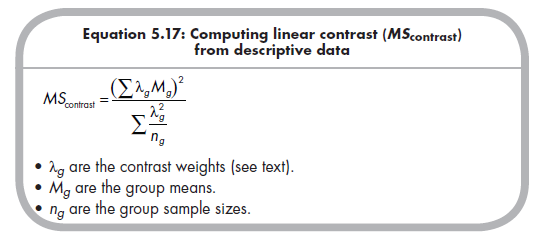
Given this squared deviation due to the contrast, one can then evaluate the statistical significance of the linear contrast, if this is of interest. This statistical significance can be evaluated as the F_contrast, which has 1 df in the numerator and df_error, or S(ng – 1), in the denominator. Regardless of whether you are interested in the significance of this contrast, the next step is to compute F_COntrast as MScontrast divided by MSwithin, where MSwithin might be reported in the primary study or can be computed as the group-size weighted average of within-group variances, S(ng sg²) / Sng.

From this F_contrast, the final step to computing an effect size from this three or more group situation is to compute r (called reffect size by Rosenthal et al., 2000)using the following equation:

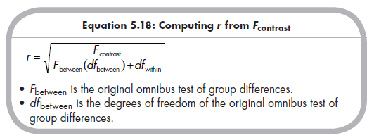
Because F_between and df_between are from the original omnibus test of group differences, primary studies typically report these values. If a study does not provide these values, you can easily compute these values from the reported sample sizes, means, and standard deviations.¹²

5.2. From df > 2 F-Ratio

Another common method of reporting results of comparisons of three or more groups in primary studies is to report the omnibus F-ratio. To compute an effect size from this F-ratio, the primary study must also report the means (but standard deviations are not necessary) of three or more groups. If the primary study does not report the means of the groups, it is not possible to compute an effect size indexing the association between the independent (grouping) and dependent (outcome) variables (note that simply using the formula for the two group ANOVAs, Equation 5.14, is not appropriate).

Computing r from reported means and an omnibus F-ratio is similar to the computation from means, standard deviations, and sample sizes described in the previous section. Specifically, you still (1) determine appropriatecontra st weights (λg); (2) compute MScontrast using Equation 5.17; and (3) compute Fcontrast for use in subsequent computations as described earlier. The difference here is that you do not use the reported group standard deviations to compute MSwithin (which is used to compute Fcontrast). If this value is reported in an ANOVA table, you can easily obtain this value. Otherwise, you must compute this MSwithin from the reported omnibus F-ratio, based on the fact that MSwithin = MSbetween/F. Although MSbetween will typically not be reported if an ANOVA table is not provided, this can be computed from the reported means from the G groups: MSbetween = S(Mg – GM)2/G – 1.

You then follow the same steps described in the previous section: (1) computing Fcontrast as MScontrast/MSwithin; (2) computing r using Equation 5.18. Thus, obtaining r from data where there are three or more groups is
similar when studies report either descriptive statistics or results of an omnibus one-way ANOVA.

5.3. Final Words Regarding Computing r from Omnibus Tests

In this section, I provide only a brief overview of computing r from the results of omnibus tests reported in primary studies. Although the simple situations I have described will likely help in most situations, others that I have not described here may emerge. My recommendation to readers who commonly encounter these situations is to first consult the book by Rosen­thal et al. (2000), which provides further details on computing r in situations I have described as well as others, including factorial designs and repeated- measures ANOVAs. These authors also describe alternative assignment of contrast weights that may be of interest.

If you encounter situations not described here or in Rosenthal et al. (2000), several options are available to you. First, I recommend consulting the literature for more recent treatments that might apply to this situation.

Computing effect sizes such as r from omnibus test results has only recently gained attention (due largely to the Rosenthal et al. book), and it is likely that more will be written on this topic. Second, you might be able to apply the logic of this approach to develop reasonable ways of computing a meaningful effect size from omnibus results. It seems safe to suggest that if you can (1) identify the amount of variance due to the desired effect (e.g., a linear rela­tion between the independent and dependent variables) and (2) determine a direction of effect, then it is possible to compute an r that indexes this effect. A third option, of course, is to request further information from the authors of the primary studies. Although this approach might deprive you of the joys of discovering ingenious ways of computing an effect size, you should remember that this is usually the most straightforward and most accurate way of obtaining the desired information.

Source: Card Noel A. (2015), Applied Meta-Analysis for Social Science Research, The Guilford Press; Annotated edition.