Analyses of Random-Effects Models

A random-effects model in meta-analysis can be estimated in four general steps: (1) estimating the heterogeneity among effect sizes, (2) estimating pop­ulation variability in effect sizes, (3) using this estimate of population vari­ability to provide random-effects weights of study effect sizes, and (4) using these random-effects weights to estimate a random-effects mean effect size and standard errors of this estimate (for significance testing and confidence intervals). I illustrate each of these steps using the example meta-analysis dataset of 22 studies providing associations between relational aggression and peer rejection. These studies, together with the variables computed to estimate the random-effects model, are summarized in following Table.

1. Estimating Heterogeneity

The first step is to estimate the heterogeneity, indexed by Q, in the same way as described in Chapter 8. As you recall, the heterogeneity (Q) is computed using Equation 8.6, reproduced here:

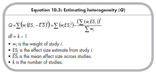
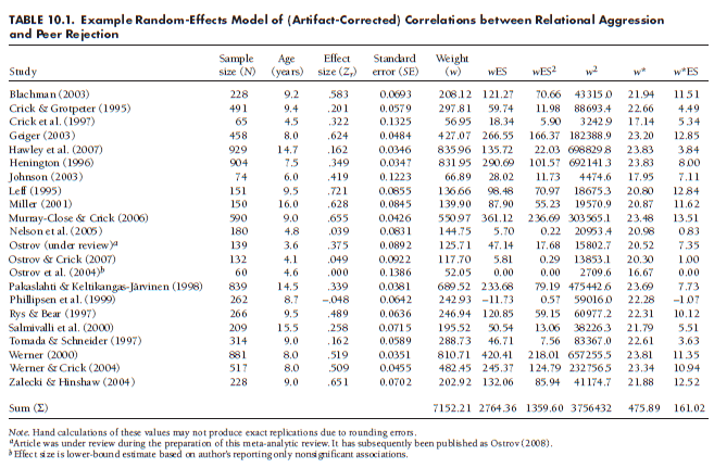
As in Chapter 8, I estimate Q in the example meta-analysis by creating three columns (variables)—w, wES, and wES²—shown in Table 10.1. This yields Q = 291.17, which is high enough (relative to a c² distribution with 21 df) to reject the null hypothesis of homogeneity and accept the alternate hypothesis of heterogeneity. Put another way, I conclude that the observed variability in effect sizes across these 22 studies is greater than expectable due to sampling fluctuation alone. This conclusion, along with other con­siderations described in Section 10.5, might lead me to use a random-effects model in which I estimate a distribution, rather than single point, of popula­tion effect sizes.

2. Estimating Population Variability

To estimate population variability, you partition the observed heterogene­ity into that expectable due to sampling fluctuations and that representing true deviations in population effect sizes. Although you can never know the extent to which one particular study’s deviation from the central tendency is due to sampling fluctuation versus its place in the distribution of popu­lation effect sizes, you can make an estimate of the magnitude of popula­tion variability based on the observed heterogeneity (total variability) and that which is expectable given the study standard errors. Specifically, you estimate population variability in effect sizes (t²) using the following equa­tion:

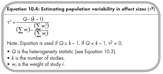
Although the denominator of this equation is not intuitive, you can understand this equation well enough by considering the numerator. Because the expected value of Q under the null hypothesis of homogeneity is equal to the degrees of freedom (k — 1), a homogeneous set of studies will result in a numerator equal to zero, and therefore the population variance in effect sizes is estimated to be zero.² In contrast, when there is considerable heterogene­ity, then Q is larger than the degrees of freedom (k – 1), and this heterogeneity beyond that expected by sampling fluctuation results in a large estimate of the population variance, t² (recalling that Q is a significance test based on the number of studies and total sample size in the meta-analysis, the denomina­tor adjusts for the sums of weights in a way that makes the estimate of popu­lation variance similar for small and large meta-analyses).

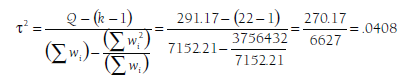
To estimate the population variance in the example meta-analysis shown in Table 10.1, I compute a new variable (column) w². I then apply Equation 10.4 to obtain

3. Computing Random-Effects Weights

Having estimated the population variability in effect sizes, the next step is to compute new, random-effects weights for each study. Before describing this computation, it is useful to consider the logic of these random-effects weights. As shown in Chapter 8, the reason for weighting effect sizes in a meta-analysis is to account for the imprecision of effect sizes, so as to give more weight to studies providing more precise effect size estimates than to those providing less precise estimates. In the fixed-effects model described in Chapter 8, imprecision in study effect sizes was assumed to be due only to the standard error of that particular effect size. This can be seen in Equation 10.1, which shows that each study’s effect size is conceptualized as a function of the single population effect size and sampling deviation from that value. As seen in Equation 10.2, random-effects models consider two sources of a deviation of effect sizes around a mean: population variance (^;, which has an estimated variance of t²) and sampling fluctuation (£;). In other words, random-effects models consider two sources of imprecision in effect size esti­mates: population variability and sampling fluctuation.

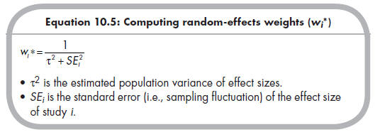
To account for these two sources of imprecision, random-effects weights are comprised of both an overall estimated population variance (t²) and a study-specific standard error (SEj) for sampling fluctuation. Specifically, random-effects weights (wj*) are computed using the following equation:

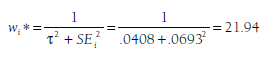
To illustrate this computation, consider the first study in Table 10.1 (Blachman, 2003). This study had a weight of 208.12 in the fixed-effects model (based on w = 1/(.0693²), allowing for rounding error). In the random- effects model, I compute a new weight as a function of the estimated popula­tion variance (t² = .0408) and the study-specific standard error (SE = .0693, to yield a study-specific sampling variance SE² = .0048):

The random-effects weights of all 22 studies are shown in Table 10.1 (second column from right). You should make two observations from these weights. First, these random-effects weights are smaller (much smaller in this exam­ple) than the fixed-effects weights. The implication of these smaller weights is that the sum of weights across studies will be smaller, and the standard error of the average mean will therefore be larger, in the random- relative to fixed-effects model. Second, although the studies still have the same relative ranking of weights using random- or fixed-effects models (i.e., studies with the largest weights for one had the largest weights for the other), the dis­crepancies in weights across studies is less for random- than for fixed-effects models. This fact impacts the relative influence of studies that are extremely large (outliers in sample size). I further discuss these and other differences between fixed- and random-effects models in Section 10.5.

4. Estimating and Drawing Inferences about Random-effects Means

The final step of the random-effects analysis is to estimate the mean effect size and to make inferences about it (through significance testing or comput­ing confidence intervals). These computations parallel those for fixed-effects
models described in Chapter 8, except that the ws of the fixed-effects mod­els are replaced with the random-effects weights, w*. To illustrate using this example of 22 studies (see the rightmost columns of Table 10.1), I compute the random-effects mean effect size (see Equation 8.2).

(which I would transform to report as the random-effects mean correlation, r = .326). Note that the random-effects mean is not identical to that of the fixed-effects mean computed in Chapter 8 (Z_r = .387, r = .367), though in this example they are reasonably close.

The standard error of this mean effect size is computed as (see Equation 8.3):

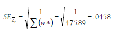
This standard error can then be used for significance testing (Z = .338 / .0458 = 7.38, p < .001) of computing confidence intervals (95% confidence inter­val of Z_r is .249 to .428, translating to a confidence interval for r of .244 to .404). Note that the standard error from the random-effects model is consid­erably larger than that computed in Chapter 8 under the fixed-effects model (.0118), resulting in lower Z values of the significance test (7.38 vs. 32.70 for the fixed-effects model) and wider confidence intervals (vs. 95% confidence interval for r of .348 to .388).

Source: Card Noel A. (2015), Applied Meta-Analysis for Social Science Research, The Guilford Press; Annotated edition.