A Structural Equation Modeling Approach to Random- and Mixed-Effects Models

In Chapter 9, I introduced an alternative approach to meta-analysis based on Cheung’s (2008) description of meta-analysis within the context of struc­tural equation modeling. Here, I extend the logic of this approach to describe how it can be used to estimate random- and mixed-effects models (follow­ing closely the presentation by Cheung, 2008). As when I introduced this approach in Chapter 9, I should caution you that this material requires a fairly in-depth understanding of SEM, and you might consider skipping this section if you do not have this background. If you do have a solid background in SEM, however, this perspective may be advantageous in two ways. First, if you are familiar with SEM programs that can estimate random slopes (e.g., Mplus, MX; I elaborate on this requirement below), then you might find it easier to use this approach than the matrix algebra required for the mixed- effects model that I described earlier. Second, as I mentioned in Chapter 9, this approach uses the FIML method of missing data management of SEM, which allows you to retain studies that have missing values of study charac­teristics that you wish to evaluate as moderators.

Next, I describe how this SEM representation of meta-analysis can be used to estimate random- and mixed-effects models. To illustrate these approaches, I consider the 22 studies reporting correlations between rela­tional aggression with rejection shown in Table 10.1.

1. Estimating Random-Effects Models

The SEM representation of random-effects meta-analysis (Cheung, 2008) parallels the fixed-effects model I described in Chapter 9 (see Figure 9.2) but models the effect size predicted by intercept path as a random slope (see, e.g., Bauer, 2003; Curran, 2003; Mehta & Neale, 2005; Muthen, 1994). In other words, this path varies across studies, which captures the between-study variance of a random-effects meta-analysis. Importantly, this SEM represen­tation can only estimate these models using software that perform random slope analyses.³

One⁴ path diagram convention for denoting randomly varying slopes is shown in Figure 10.2. This path diagram contains the same representation of regressing the transformed effect size onto the transformed intercept as does the fixed-effects model of Chapter 9 (see Figure 9.1). However, there is a small circle on this path, which indicates that this path can vary randomly across cases (studies). The label u next to this circle denotes that the newly added piece to the path diagram—the latent construct labeled u—represents the random effect. The regression path (b0) from the constant (i.e., the tri­angle with “1” in the middle) to this construct captures the random-effects mean. The variance of this construct (m, using Cheung’s 2008 notation) is the estimated between-study variance of the effect size (what I had previously called t²).

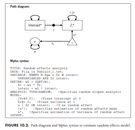
To illustrate, I fit the data from 22 studies shown in Table 10.1 under an SEM representation of a random-effects model. As I described in Chap­ter 9, the effect sizes (Z_r) and intercepts (the constant 1) of each study are transformed by multiplying these values by the square root of the study’s weight (Equation 9.7). This allows each study to be represented as an equally weighted case in the analysis, as the weighting is accomplished through these transformations.

The Mplus syntax shown in Figure 10.2 specifies that this is a random- slopes analysis by inserting the “TYPE=RANDOM” command, specifying that U represents the random effect with estimated mean and variance. The mean of U is the random-effects mean of this meta-analysis; here, the value was estimated to be 0.369 with a standard error of .049. This indicates that the random-effects mean Z_r is .369 (equivalent r = .353) and statistically sig­nificant (Z = .369/.049 = 7.53, p < .01; alternatively, I could compute confi­dence intervals). The between-study variance (t²) is estimated as the variance of U; here, the value is .047.

The random-effects mean and estimated between-study variance obtained using this SEM representation are similar to those I reported earlier (Section 10.2). However, they are not identical (and the differences are not due solely to rounding imprecision). The differences in these values are due to the dif­ference in estimation methods used by these two approaches; the previously described version used least squares criteria, whereas the SEM representa­tion used maximum likelihood (the most common estimation criterion for SEM). To my knowledge, there has been no comprehensive comparison of which estimation method is preferable for meta-analysis (or—more likely— under what conditions one estimator is preferable to the other). Although I encourage you to watch for future research on this topic, it seems reasonable to conclude for now that results should be similar, though not identical, for either approach.

2. Estimating Mixed-Effects Models

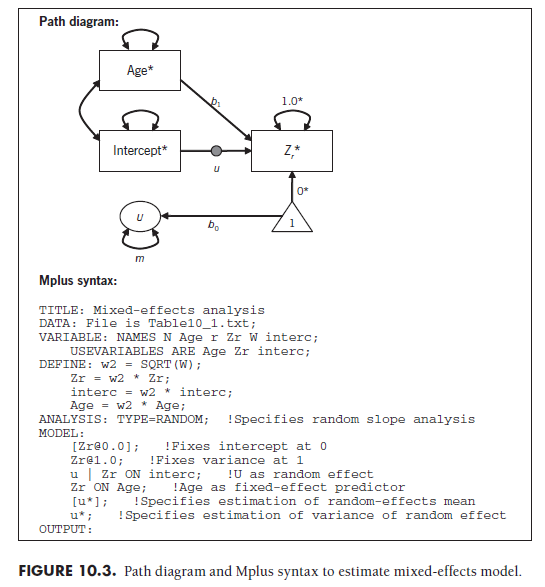
As you might anticipate, this SEM approach (if you have followed the mate­rial so far) can be rather easily extended to estimate mixed-effects models, in which fixed-effects moderators are evaluated in the context of random between-study heterogeneity. To evaluate mixed-effects models in an SEM framework, you simply build on the random-effects model (in which the transformed intercept predicting transformed effect size slope randomly var­ies across studies) by adding transformed study characteristics (moderators) as fixed predictors of the effect size.

I demonstrate this analysis using the 22 studies from Table 10.1, in which I evaluate moderation by sample age while also modeling between- study variance (paralleling analyses in Section 10.3). This model is graphi­cally shown in Figure 10.3, with accompanying Mplus syntax. As a reminder, the effect size and all predictors (e.g., age and intercept) are transformed for each study by multiplying by the square root of the study weight (Equation 9.7). To evaluate the moderator, you evaluate the predictive path between the coded study characteristic (age) and the effect size. In this example, the value was estimated as b1 = .013, with a standard error of .012, so it was not statistically significant (Z = .013/012 = 1.06, p = .29). These results are simi­lar to those obtained using the iterative matrix algebra approach I described in Section 10.3, though they will not necessarily be identical given different estimator criteria.

3. Conclusions Regarding SEM Representations

As with fixed-effects moderator analyses, the major advantage of estimating mixed-effects meta-analytic model in the SEM framework (Cheung, 2008) is the ability to retain studies with missing predictors (i.e., coded study char­acteristics in the analyses). If you are fluent with SEM, you may even find it easier to estimate models within this framework than using the other approaches.

You should, however, keep in mind several cautions that arise from the novelty of this approach. It is likely that few (if any) readers of your meta­analysis will be familiar with this approach, so the burden falls on you to describe it to the reader. Second, the novelty of this approach also means that some fundamental issues have yet to be evaluated in quantitative research. For instance, the relative advantages of maximum likelihood versus least squares criteria, as well as modifications that may be needed under certain condi-tions (e.g., restricted maximum likelihood or other estimators with small numbers of studies) represent fundamental statistical underpinnings of this approach that have not been fully explored (see Cheung, 2008). Nevertheless, this representation of meta-analysis within SEM has the potential to merge to analytic approaches with long histories, and there are many opportuni­ties to apply the extensive tools from the SEM field in your meta-analyses. For these reasons, I view the SEM representation as a valuable approach to consider, and I encourage you to watch the literature for further advances in this approach.

Source: Card Noel A. (2015), Applied Meta-Analysis for Social Science Research, The Guilford Press; Annotated edition.