Mixed-Effects Models

Mixed-effects models, sometimes called conditionally random models, com­bine the (fixed-effects) moderator analyses of Chapter 9 with the estimation of variance in population effect sizes (random-effects) described earlier in this chapter. These models are useful when you want to evaluate moderators in meta-analysis, and you (1) either want the generalizability provided by random-effects models, or (2) fixed-effects moderator analyses (as described in Chapter 9) indicate significant residual heterogeneity (i.e., Q_withi_n in ANOVA framework or Q_residual in regression framework).

Mixed-effects models follow the logic of moderator analyses within a general regression framework (see Chapter 9.3). However, these models include additional terms representing population variability in effect sizes, above and beyond systematic variability accounted for by moderators as well as sampling fluctuations. The general equation for mixed-effects models can be represented by the following equation:

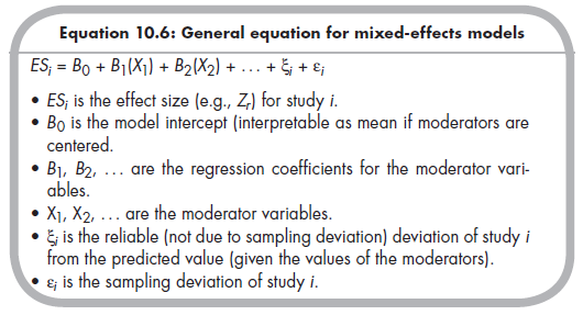
Unfortunately, estimating mixed-effects models requires intensive, fairly complex methods. Specifically, estimating mixed-effects models requires iterative matrix algebra (or analysis within an SEM framework, which I present in the next section). I describe and illustrate this estimation using the example meta-analysis (Table 10.1) of 22 studies next, evaluating sample age as a moderator in the context of between-study heterogeneity. However, I forewarn you that the material presented in the remainder of this section is complex.

Before describing the estimation of mixed-effects models, however, it is useful to begin by describing the analysis of a moderator variable within a fixed-effects framework using matrix algebra. After describing this fixed- effects framework, I will describe and illustrate the estimation of mixed- effects models through an iterative matrix algebra.

1. Matrix Algebra of Fixed-effects Moderator Analysis

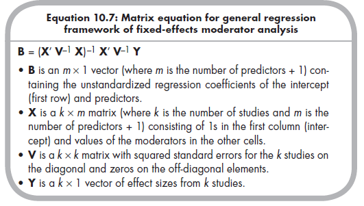
The general regression framework of analyzing moderators within the fixed- effects context (Section 9.3) can be solved using matrix algebra given the fol­lowing equation (from Overton, 1998):

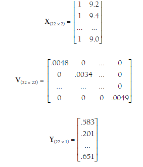
To illustrate this computation with the example meta-analysis of 22 studies summarized in Table 9.4, in which I am interested in whether age moderates the association between relational aggression and peer rejection the following matrices are created:

Working through the matrix algebra to solve Equation 10.7 (using any basic matrix algebra calculator) yields the following matrix:

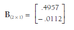
The value in the first row (.4957) represents the intercept, and the value in the second row (-.0112) represents the regression coefficient of the first predictor, age (additional rows would contain additional regression coeffi­cients if I had included additional predictors).

Variances of these estimates of the regression coefficients are obtained via the diagonal of the m X m matrix, = (X’ V^-1 X)^-1. In this example,

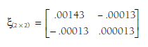
Standard errors of these estimates can be computed as the square roots of these values. In this example, the standard error of the estimate of the intercept is .0378 (V.00143), and the standard error of the regression coeffi­cient (i.e., moderation by age) is .0037 (V.000013). Note that these values are identical to those reported in Chapter 9.

2. Estimation of Mixed-Effects Models

Mixed-effects models are estimated iteratively (see simulation by Overton, 1998)—that is, through a series of estimations of B using V, recomputing the weights in this new solution to yield a new set of values for V, and then using these new values of V to reestimate B, with the process repeating itself until a certain standard of convergence is reached (see Overton, 1998).

2.1. Iteration I

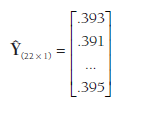
The fixed-effects estimation of B serves as the first iteration. Here, the matrix of weights (V) assumes that t² = 0. From this solution, you compute the model predicted values of the effect size for each study using the following matrix equation (Overton, 1998):

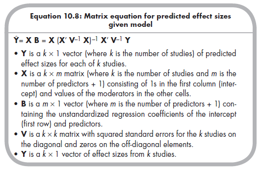
To illustrate using the example meta-analysis of 22 studies:

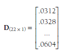
You then consider the discrepancies between the actual (observed) effect sizes of the studies and these predicted (by the intercept and any moderators) values. Specifically, you compute a matrix, D, representing k squared devia­tions that serve as estimates of the population conditional variance (t²):

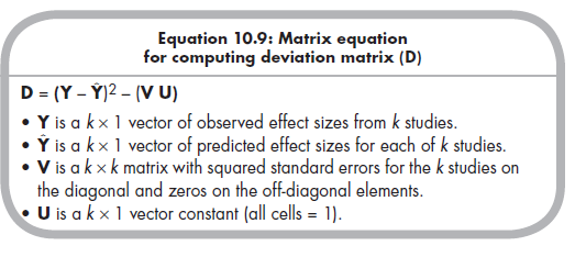
To illustrate with the example meta-analysis, the D from the first itera­tion (i.e., fixed-effects model) is:

You then take the weighted average of these k estimates (22 in this exam­ple) in D to provide a single estimate of the population conditional variance (t²) using the following equation:

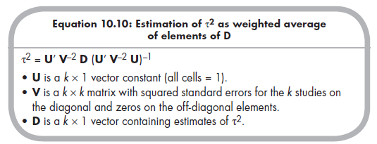
Applying this equation to the example data of 22 studies yields an esti­mated t² = .0240.

2.2. Subsequent Iterations

This estimated t² is now added to the standard errors of each study (sam­pling fluctuations), such that Vj* = t² + SEj². For example, the first study in the example dataset would receive the value that V]* = .0240 + (.0693)² = .0288. These k Vj*s would be entered in the diagonal of the new matrix V* for iteration 2. Equation 10.7 is then recomputed using V* to yield a new set of estimated regression coefficients. In the example data, these values at the second iteration are Bq = .2700 and B] = .0112.

These regression coefficients are used to compute new predicted scores using Equation 10.8, new discrepancy scores are estimated, and a new D is computed using Equation 10.9 (note that at this step, the original V is used because you want to subtract out only the sampling variance). The t² is then
reestimated using Equation 10.10 (using V*). This process continues until the estimated t² changes minimally between successive iterations. Although the convergence criteria have not been well studied, Overton (1998, citing Erez et al., 1996) suggested that A t² less than 10^-10 is adequate and usually achieved by the seventh iteration. Using the example meta-analysis of 22 studies, I achieved this level of convergence in six iterations.

Overton (1998) has shown that a small correction for t² following the final iteration improves the estimation of mixed-effects models. This correc­tion multiplies the obtained t² by k/(k – m), where k = the number of studies and m = number of predictors (including constant). Applying this correction within the example meta-analysis yields the final estimates of t² = .0499, with regression weights estimated as B0 = .2548 (intercept) and B1 = .0128 (moderating effect of age).

Source: Card Noel A. (2015), Applied Meta-Analysis for Social Science Research, The Guilford Press; Annotated edition.