In Sections 10.1 and 10.2, I have presented the random-effects model for estimating mean effect sizes, which can be contrasted with the fixed-effects model I described in Chapter 8. I have also described (Section 10.3) mixed- effects models, in which (fixed) moderators are evaluated in the context of conditional random heterogeneity; this section can be contrasted with the fixed-effects moderator analyses of Chapter 9. An important question to ask now is which of these models you should use in a particular meta-analysis. At least five considerations are relevant: the types of conclusions you wish to draw, the presence of unexplained heterogeneity among the effect sizes in your meta-analysis, statistical power, the presence of outliers, and the complexity of performing these analyses. I have arranged these in order from most to least important, and I elaborate on each consideration next. I conclude this section by describing the consequences of using an inappropriate model; these consequences serve as a further set of considerations in selecting a model.
Perhaps the most important consideration in deciding between a fixed- versus random-effects model, or between a fixed-effects model with moderators versus a mixed-effects model, is the types of conclusions you wish to draw. As I described earlier, conclusions from fixed-effects models are limited to only the sample of studies included in your meta-analysis (i.e., “these studies show . . . ” type conclusions), whereas random- and mixed-effects models allow more generalizable conclusions (i.e., “the research shows . . . ” or “there is…” type of conclusions). Given that the last-named type of conclusions are more satisfying (because they are more generalizable), this consideration typically favors the random- or mixed-effects models. Regardless of which type of model you select, however, it is important that you frame your conclusions in a way consistent with your model.
A second consideration is based on the empirical evidence of unexplained heterogeneity. By unexplained heterogeneity, I mean two things. First, in the absence of moderator analysis (i.e., if just estimating the mean effect size), finding a significant heterogeneity (Q) test (see Chapter 8) indicates that the heterogeneity among effect sizes cannot be explained by sampling fluctuation alone. Second, if you are conducting fixed-effects moderator analysis, you should examine the within-group heterogeneity (Qwithin; for ANOVA analogue tests) or residual heterogeneity (Qresidual; for regression analog tests). If these are significant, you conclude that there exists heterogeneity among effect sizes not systematically explained by the moderators.5 In both situations, you might use the absence versus presence of unexplained heterogeneity to inform your choice between fixed- versus random- or mixed-effects models (respectively). Many meta-analysts take this approach. However, I urge you to not make this your only consideration because the heterogeneity (i.e., Q) test is an inferential test that can vary in statistical power. In meta-analyses with many studies that have large sample sizes, you might find a significant residual heterogeneity that is trivial, whereas a meta-analysis with few studies having small sample sizes might fail to detect potentially meaningful heterogeneity. For this reason, I recommend against basing your model decision only on empirical findings of unexplained heterogeneity.
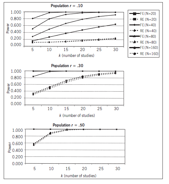
A third consideration is the relative statistical power of fixed- versus random-effects models (or fixed-effects with moderators versus mixed- effects models). The statistical power of a meta-analysis depends on many factors—number of studies, sample sizes of studies, degree to which effect sizes must be corrected for artifacts, magnitude of population variance in effect size, and of course true mean population effect size. Therefore, it is not a straightforward computation (see e.g., Cohn & Becker, 2003; Field, 2001; Hedges & Pigott, 2001, 2004). However, to illustrate this difference in power between fixed- and random-effects models, I have graphed some results of a simulation by Field (2001), shown in Figure 10.4. These plots make clear the greater statistical power of fixed-effects versus random-effects models. More generally, fixed-effects analyses will always provide as high (when t2 = 0) or higher (when t2 > 0) statistical power than random-effects models. This makes sense in light of my earlier observation that the random-effects weights are always smaller than the fixed-effects weights; therefore, the sum of weights is smaller and the standard error of the average effect size is larger for random- than for fixed-effects models. Similarly, analysis of moderators in fixed-effects models will provide as high or higher statistical power as mixed-effects models. For these reasons, it may seem that this consideration would always favor fixed-effects models. However, this conclusion must be tempered by the inappropriate precision associated with high statistical power when a fixed-effects model is used inappropriately in the presence of substantial variance in population effect sizes (see below). Nevertheless, statistical power is one important consideration in deciding among models: If you have questionable statistical power (small number of studies and/or small sample sizes) to detect the effects you are interested in, and you are comfortable with the other considerations, then you might choose a fixed- effects model.
The presence of studies that are outliers in terms of either their effect sizes or their standard errors (e.g., sample sizes) is better managed in ran-dom- than fixed-effects models. Outliers consisting of studies that have extreme effect sizes have more influence on the estimated mean effect size in fixed-effects analysis because the analyses—to anthropomorphize—must “move the mean” substantially to fall within the confidence interval of the extreme effect size (see top of Figure 10.1). In contrast, studies with extreme effect sizes impact the population variance (t2) more so than the estimated mean effect size in random-effects models. Considering the bottom of Figure 10.1, you can imagine that an extreme effect size can be accommodated by widening the spread of the population effect size distribution (i.e., increasing the estimate of t) in a random-effects model.
A second type of outlier consists of studies that are extreme in their sample sizes, especially those with much larger sample sizes than other studies. Because sample size is strongly connected to the standard error of the study’s effect size, and these standard errors in turn form the weight in fixed-effects models (see Chapter 8), you can imagine that a study with an extremely large sample could be weighted much more heavily than other studies. For example, in the 22 study meta-analyses I have presented (see Table 10.1), four studies with large samples (Hawley et al., 2007; Henington, 1996; Pakaslahti and Keltikangas-Jarvinen, 1998; Werner, 2000) comprise 44% of the total weight in the fixed-effects analysis (despite being only 18% of the studies) and are given 13 to 16 times the weight of the smallest study (Ostrov, Woods, Jansen, Casas, & Crick, 2004). Although I justified the use of weights in Chapter 8, this degree of weighting some studies far more than others might be too undemocratic (and I have seen meta-analyses with even more extreme weighting, with single studies having more weight than all other studies combined). As I have mentioned, random-effects models reduce these discrepancies in weighting. Specifically, because a common estimate of t2 is added to the squared standard error for each study, the weights become more equal across studies as t2 becomes larger. This can be seen by inspecting the random-effects weights (w*) in Table 10.1: Here the largest study is only weighted 1.4 times the smallest study. In sum, random-effects models, to the extent that t2 is large, use weights that are less extreme, and therefore random- (or mixed-) effects models might be favored in the presence of sample size outliers.
Perhaps the least convincing consideration is the complexity of the models (the argument is so unconvincing that I would not even raise it if it was not so commonly put forward). The argument is that fixed-effects models, whether for only computing mean effect sizes (Chapter 8) or for evaluating moderators (Chapter 9) are far simpler than random- and mixed-effects models. Although simplicity is not a compelling rationale for a model (and a rationale that will not go far in the publication process), I acknowledge that you should be realistic in considering how complex of a model you can use and report. I suspect that most readers will be able to perform computations for random-effect models, so if you are not analyzing moderators and the other considerations point you toward this model, I encourage you to use it. Mixed- effects models, in contrast, are more complex and might not be tractable for many readers. Because less-than-optimal answers are better than no answers at all, I do think it is reasonable to analyze moderators within a fixed-effects model if this is all that you feel you can do—with the caveat that you should recognize the limitations of this model. Even better, however, is for you to enlist the assistance of an experienced meta-analyst who can help you with more complex—and more appropriate—models.
At this point, you might see some advantages and disadvantages to each type of model, and you might still feel uncertain about which model to choose. I think this decision can be aided by considering the consequences of choosing the “wrong” model. By “wrong” model, I mean that you choose (1) a random- or mixed-effects model when there is no population variability among effect sizes, or (2) a fixed-effects model when there really exists substantial population variability among effect sizes. In the first situation, using random-effects models in the absence of population variability, there is little negative consequence other than a little extra work. Random- and mixed- effects models will yield similar results as fixed-effects models when there is little population variability in effect sizes (e.g., because estimated t2 is close to zero, Equation 10.2 functionally reduces to Equation 10.1). If you decide on a random- (or mixed-) effects model only to find little population variability in effect sizes, you still have the advantage of being able to make generaliz- able conclusions (see the first consideration above). In contrast, the second type of inappropriate decision (using a fixed-effects model in the presence of unexplained population variability) is problematic. Here, the failure to model this population variability leads to conclusions that are inappropriately precise—in other words, artificially high significance tests and overly narrow confidence intervals.
In conclusion, random-effects models offer more advantages than fixed- effects models, and there are no disadvantages to using random-effects models in the absence of population variability in effect sizes. For this reason, I generally recommend random-effects models when the primary goal is estimated and drawing conclusions about mean effect sizes. When the focus of your meta-analysis is on evaluating moderators, then my recommendations are more ambivalent. Here, mixed-effects models provide optimal results, but the complexity of estimating them might not always be worth the effort unless you are able to enlist help from an experienced meta-analyst. For moderator analyses, I do view fixed-effects models as acceptable, provided you examine unexplained (residual) heterogeneity and are able to show that it is either not significant or small in magnitude.6
Source: Card Noel A. (2015), Applied Meta-Analysis for Social Science Research, The Guilford Press; Annotated edition.
25 Aug 2021
25 Aug 2021
25 Aug 2021
25 Aug 2021
24 Aug 2021
24 Aug 2021