1. Sufficient Statistics for Multivariate Analyses
As you may recall (fondly or not) from your multivariate statistics courses, nearly all multivariate analyses do not require the raw data. Instead, you can perform these analyses using sufficient statistics—summary information from your data that can be inserted into matrix equations to provide estimates of multivariate parameters. Typically, the sufficient statistics are the variances and covariances among the variables in your multivariate analysis, along with some index of sample size for computing standard errors of these parameter estimates. For some analyses, you can instead use correlation to obtain standardized multivariate parameter estimates. Although the analysis of correlation matrices, rather than variance/covariance matrices, is often less than optimal, a focus on correlation matrices is advantageous in the context of multivariate meta-analysis for the same reason that correlations are generally preferable to covariances in meta-analysis (see Chapter 5). I next briefly summarize how correlation matrices can be used in multivariate analyses, focusing on multiple regression, exploratory factor analysis, and confirmatory factor analysis. Although these represent only a small sampling of possible multivariate analyses, this focus should highlight the wide range of possibilities of using multivariate meta-analysis.
1.1. Multiple Regression
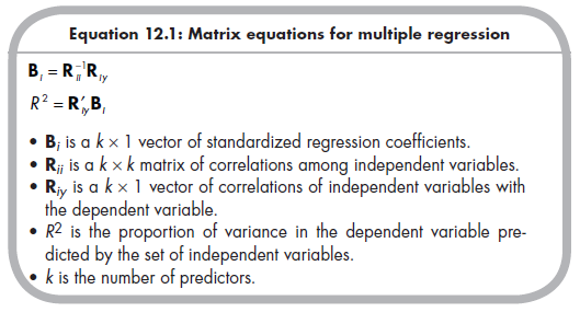
Multiple regression models fit linear equations between a set of predictors (independent variables) and a dependent variable. Of interest are both the unique prediction each independent variable has to the dependent variable above and beyond the other predictors in the model (i.e., the regression coefficient, B) and the overall prediction of the set (i.e., the variance in the dependent variable explained, R2). Both the standardized regression coefficients of each predictor and overall variance explained (i.e., squared multiple correlation, R2) can be estimated from (1) the correlations among the independent variables (a square matrix, R^, with the number of rows and columns equal to the number of predictors), and (2) the correlations of each independent variable with the dependent variable (a column vector, Rjy, with the number of rows equal to the number of predictors, using the following equations1 (Tabachnick & Fidell, 1996, p. 142):
1.2. Exploratory Factor Analys/s
Exploratory factor analysis (EFA) is used to extract a parsimonious set of factors that explain associations among a larger set of variables. This approach is commonly used to determine (1) how many factors account for the associations among variables, (2) the strengths of associations of each variable on a factor (i.e., the factor loadings), and (3) the associations among the factors (assuming oblique rotation). For each of these goals, exploratory factor analysis is preferred to principal components analysis (PCA; see, e.g., Widaman, 1993, 2007), so I describe EFA only. I should note that my description here is brief and does not delve into the many complexities of EFA; I am being brief because I seek only to remind you of the basic steps of EFA without providing a complete overview (for more complete coverage, see Cudeck & MacCallum, 2007).
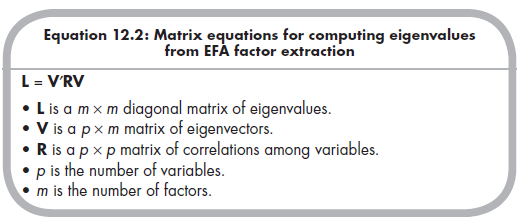
Although the matrix algebra of EFA can be a little daunting, all that is initially required is the correlation matrix (R) among the variables, which is a square matrix of p rows and columns (where p is the number of variables). From this correlation matrix, it is possible to compute a matrix of eigenvectors, V, which has p rows and m columns (where m is the number of factors).2
To determine the number of factors that can be extracted, you extract the maximum number of factors3 and then examine the resulting eigenvalues contained in the diagonal matrix (m X m) L:
You decide on the number of factors to retain based on the magnitudes of the eigenvalues contained in L. A minimum (i.e., necessary but not sufficient) threshold is known as Kaiser’s (1970) criterion, which states that the eigenvalue is greater than 1.0. Beyond this criterion, it is common to rely on a scree plot, sometimes with parallel analysis, as well as considering the inter- pretability of rival solutions, to reach a final determination of the number of factors to retain.
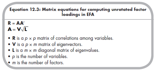
The analysis then proceeds with a specified number of factors (i.e., some fixed value of m that is less than p). Here, the correlation matrix (R) is expressed in terms of a matrix of unrotated factor loadings (A), which are themselves calculated from the matrices of eigenvectors (V) and eigenvalues (L):
In order to improve the interpretability of factor loadings (contained in the matrix A), you typically apply a rotation of some sort. Numerous rotations exist, with the major distinction being between orthogonal rotations, in which the correlations among factors are constrained to be zero, versus oblique rotations, in which nonzero correlations among factors are estimated. Oblique rotations are generally preferable, given that it is rare in social sciences for factors to be truly orthogonal. However, oblique rotations are also more computationally intensive (though this is rarely problematic with modern computers) and can yield various solutions using different criteria, given that you are attempting to estimate both factor loadings and factor intercorrelations simultaneously. I avoid the extensive consideration of alternative estimation procedures by simply stating that the goal of each approach is to produce a reproduced (i.e., model implied) correlation matrix that closely corresponds (by some criterion) to the actual correlation matrix (R). This reproduced matrix is a function of (1) the pattern matrix (A), which here (with oblique rotation) represents the unique relations of variable with factors (controlling for associations among factors), and (2) the factor correlation matrix (F), which represents the correlations among the factors4:
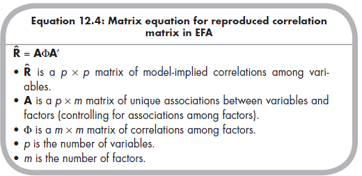
When the reproduced correlation matrix (R) adequately reproduces the observed correlation matrix (R), the analysis is completed. You then interpret the values within the pattern matrix (A) and matrix of factor correlations (F) to address the second and third goals of EFA described above.
1.3. Confirmatory Factor Analysis
In many cases, it may be more appropriate to rely on a confirmatory, rather than an exploratory, factor analysis. A confirmatory factor analysis (CFA) is estimated by fitting the data to a specified model in which some factor loadings (or other parameters, such as residual covariances among variables) are specified as fixed to zero versus freely estimated. Such a model is often a more realistic representation of your expected factor structure than is the EFA.5
Like the EFA, the CFA estimates associations among factors (typically called “constructs” or “latent variables” in CFA) as well as strengths of associations between variables (often called “indicators” or “manifest variables” in CFA) and constructs. These parameters are estimated as part of the general CFA matrix equation6:
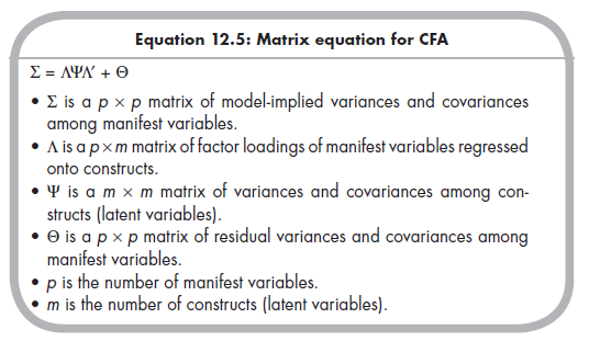
To estimate a CFA, you place certain constraints on the model to set the scale of latent constructs (see Little, Slegers, & Card, 2006) and ensure identification (see Kline, 2010, Ch. 6). For example, you might specify that there is no factor loading of a particular indicator on a particular construct (vs. an EFA, in which this would be estimated even if you expected the value to be small). Using Equation 12.5, a software program (e.g., Lisrel, EQS, Mplus) is used to compute values of factor loadings (values within the A matrix), latent variances and covariances (values within the ¥ matrix), and residual variances (and sometimes residual covariances; values within the 0 matrix) that yield a model implied variance/covariance matrix, S. The values are selected so that this model-implied matrix closely matches the observed (i.e., from the data) variances and covariance matrix (S) according to some criterion (most commonly, the maximum likelihood criterion minimizing a fit function). For CFA of primary data, the sufficient statistics are therefore the variances and covariances comprising S; however, it is also possible to use correlation coefficients such as would be available from meta-analysis to fit CFAs (see Kline, 2010, Ch. 7).7
2. The Logic of Meta-Analytically Deriving Sufficient Statistics
The purpose of the previous section was not to fully describe the matrix equations of multiple regression, EFA, and CFA. Instead, I simply wish to illustrate that a range of multivariate analyses can be performed using only correlations. Other multivariate analyses are possible, including canonical correlations, multivariate analysis of variance or covariance, and structural equation modeling. In short, any analysis that can be performed using a correlation matrix as sufficient information can be used as a multivariate model for meta-analysis.
The “key” of multivariate meta-analysis then is to use the techniques of meta-analysis described throughout this book to obtain average correlations from multiple studies. Your goal is to compute a meta-analytic mean correlation for each of the correlations in a matrix of p variables. Therefore, your task in a multivariate meta-analysis is not simply to perform one metaanalysis to obtain one correlation, but to perform multiple meta-analyses to obtain all possible correlations among a set of variables. Specifically, the number of correlations in a matrix of p variables is equal to p(p —1)/2. This correlation matrix (R) of these mean correlations is then used in one of the multivariate analyses described above.
3. The challenges of using Meta-Analytically deriving Sufficient Statistics
Although the logic of this approach is straightforward, several complications arise (see Cheung & Chan, 2005a). The first is that it is unlikely that every study that provides information on one correlation will provide information on all correlations in the matrix. Consider a simple situation in which you wish to perform some multivariate analysis of variables X, Y, and Z. Study 1 might provide all three correlations Oxy, rxz, and ryz). However, Study 2 did not measure Z, so it only provides one correlation Oxy); Study 3 failed to measure Y and so also provides only one correlation (rxz); and so on. In other words, multivariate meta-analysis will almost always derive different average correlations from different subsets of studies.
This situation poses two problems. First, it is possible that different correlations from very different sets of studies could yield a correlation matrix that is nonpositive definite. For example, imagine that three studies reporting txy yield an average value of .80 and four studies reporting rxz yield an average value of .70. However, the correlation between Y and Z is reported in three different studies, and the meta-analytic average is -.50. It is not logically possible for there to exist, within the population, a strong positive correlation between X and Y, a strong positive correlation between X and Z, but a strong negative correlation between Y and Z.8 Most multivariate analyses cannot use such nonpositive definite matrices. Therefore, the possibility that such nonpositive definite matrices can occur if different subsets of studies inform different correlations within the matrix represents a challenge to multivariate meta-analysis.
Another challenge that arises from the meta-analytic combination of different studies for different correlations within the matrix has to do with uncertainty about the effective sample size. Although many multivariate analyses can provide parameter estimates from correlations alone, the standard errors of these estimates (for significance testing or constructing confidence intervals) require knowledge of the sample size. When the correlations are meta-analytically combined from different subsets of studies, it is unclear what sample size should be used (e.g., the smallest sum of participants among studies for one of the correlations; the largest sum; or some average?).
A final challenge of multivariate meta-analysis is how we manage heterogeneity among studies. By computing a matrix of average correlations, we are implicitly assuming that one value adequately represents the populations of effect sizes. However, as I discussed earlier, it is more appropriate to test this homogeneity (vs. heterogeneity; see Chapter 8) and to model this population heterogeneity in a random-effects model if it exists (see Chapter 9). Only one of the two approaches I describe next can model between-study variances in a random-effects model.
Source: Card Noel A. (2015), Applied Meta-Analysis for Social Science Research, The Guilford Press; Annotated edition.
24 Aug 2021
24 Aug 2021
25 Aug 2021
24 Aug 2021
25 Aug 2021
24 Aug 2021