Analysis of Variance with SPSS – Problem 10.1: One-Way (or Single Factor) ANOVA

In this problem, you will examine a statistical technique for comparing two or more independent groups on the dependent variable. The appropriate statistic, called One-Way ANOVA, compares the means of the samples or groups in order to make inferences about the population means. One­way ANOVA also is called single factor analysis of variance because there is only one independent variable or factor. The independent variable has nominal levels or a few ordered levels. The overall ANOVA test does not take into account the order of the levels, but additional tests (contrasts) can be done that do consider the order of the levels. More information regarding contrasts can be found in Leech et al. (in press).

Remember that, in Chapter 9, we used the independent samples t test to compare two groups (males and females). The one-way ANOVA may be used to compare two groups, but ANOVA is necessary if you want to compare three or more groups (e.g., three levels of father’s education) in a single analysis. Review Fig. 6.1 and Table 6.1 to see how these statistics fit into the overall selection of an appropriate statistic.

Assumptions of ANOVA

1. Observations are independent. The value of one observation is not related to any other observation. In other words, one person’s score should not provide any clue as to how any of the other people would score. Each person is in only one group and has only one score on each measure; there are no repeated or within-subjects measures.
2. Variances on the dependent variable are equal across groups.
3. The dependent variable is normally distributed for each group.

Because ANOVA is robust, it can be used when variances are only approximately equal if the number of subjects in each group is approximately equal. ANOVA also is robust if the dependent variable data are approximately normally distributed. Thus, if assumption #2, or, even more so, #3 is not fully met, you may still be able to use ANOVA. There are also several choices of post hoc tests to use depending on whether the assumption of equal variances has been violated.

Dunnett’s C and Games-Howell are appropriate post hoc tests if the assumption of equal variances is violated.

10.1 Are there differences among the three father’s education revised groups on grades in h.s., visualization test scores, and math achievement?

We will use the One-Way ANOVA procedure because we have one independent variable with three levels. We can do several one-way ANOVAs at a time so we will do three ANOVAs in this problem, one for each of the three dependent variables. Note that you could do MANOVA (see Fig. 6.1) instead of three ANOVAs, especially if the dependent variables are correlated and conceptually related, but that is beyond the scope of this book. See our companion book (Leech et al., in press).

To do the three one-way ANOVAs, use the following commands:

• Analyze → Compare Means → One-Way ANOVA…
• Move grades in h.s., visualization test, and math achievement into the Dependent List: box in Fig. 10.1.
• Click on father’s educ revised and move it to the Factor (independent variable) box.
• Click on Options to get Fig. 10.2.
• Under Statistics, choose Descriptive and Homogeneity of variance test.

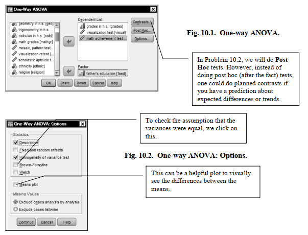
• Under Missing Values, choose Exclude cases analysis by analysis.
• Click on Continue then OK. Compare your output to Output 10.1.

Output 10.1: One-Way ANOVA

ONEWAY grades visual mathach BY faedRevis

/STATISTICS DESCRIPTIVES HOMOGENEITY

/MISSING ANALYSIS.

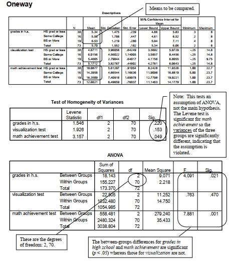
The between-groups differences for grades in high school and math achievement are significant (p < .05) whereas those for visualization are not.

Interpretation of Output 10.1

The first table, Descriptives, provides familiar descriptive statistics for the three father’s education groups on each of the three dependent variables (grades in h.s., visualization test, and math achievement) that we requested for these analyses. Remember that, although these three dependent variables appear together in each of the tables, we have really computed three separate one-way ANOVAs.

The second table (Test of Homogeneity of Variances) provides the Levene’s test to check the assumption that the variances of the three father’s education groups are equal for each of the dependent variables. Notice that for grades in h.s. (p = .220) and visualization test (p = .153) the Levene’s tests are not significant. Thus, the assumption is not violated. However, for math achievement, p = .049; therefore, the Levene’s test is significant and thus the assumption of equal variances is violated. In this latter case, we could use the similar nonparametric test (Kruskal- Wallis). Or, if the overall F is significant (as you can see it was in the ANOVA table), you could use a post hoc test designed for situations in which the variances are unequal. We will do the latter in Problem 2 and the former in Problem 3 for math achievement.

The ANOVA table in Output 10.1 is the key table because it shows whether the overall Fs for these three ANOVAs were significant. Note that the three father’s education groups differ significantly on grades in h.s. and math achievement but not visualization test. When reporting these findings one should write, for example, F (2, 70) = 4.09, p = .021, for grades in h.s. The 2, 70 (circled for grades in h.s. in the ANOVA table) are the degrees of freedom (df) for the between-groups “effect” and within-groups “error,” respectively. F tables also usually include the mean squares, which indicate the amount of variance (sums of squares) for that “effect” divided by the degrees of freedom for that “effect.” You also should report the means (and SDs) so that one can see which groups were high and low. Remember, however, that if you have three or more groups you will not know which specific pairs of means are significantly different unless you do a priori (beforehand) contrasts (see Fig. 10.1) or post hoc tests, as shown in Problem 10.2. We provide an example of appropriate APA-format tables and how to write about these ANOVAs after Problem 10.2.

Source: Morgan George A, Leech Nancy L., Gloeckner Gene W., Barrett Karen C.

(2012), IBM SPSS for Introductory Statistics: Use and Interpretation, Routledge; 5th edition; download Datasets and Materials.