Problem 12.3: Unconditional Individuals-Nested-in-Schools Model with SPSS

For this problem, you will need to retrieve a new data set, HSB12.sav (not HSBdataNew.sav or any of the other datasets).

This data set was downloaded from http://www.ats.ucla.edu/stat/paperexamples/singer/ with permission of Professor Judith D. Singer, and it was also analyzed in Raudenbush & Bryk (2002) and Singer (1998). It involves much of the same HSB data that we have used in other chapters, except that this version of the dataset includes information about which school students attended, students’ SES, average school SES, information about the type of school, and so on.

This data set includes 7185 students whose data are nested within 160 different schools. Mathach has a mean of 12.75 and SD = 6.88 for the whole sample; however, the mean mathach varies across schools from 4.24 to 19.09, and the SD for mathach ranges from 3.88 to 8.48. The question we ask in this problem is whether there is sufficient variability within and/or between schools that we might want to try to explain that variability.

Let’s answer the following question:

12.3 Is there significant variability within and/or among schools in the average mathach?

• First, click on Analyze → Mixed Models → Linear.
• Next, highlight school and move it into the Subjects: box to get 12.11.

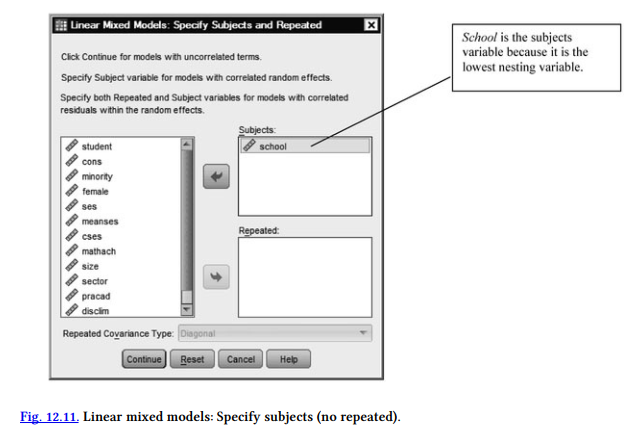
• Click on Continue.
• Highlight mathach and move it into the Dependent Variable: box. Do not put in any factors or covariates for this unconditional model. Your window should look like Fig. 12.12.

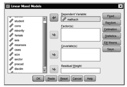
Fig. 12.12. Linear mixed models.

• Click on Fixed to get 12.13.
• In Figure 12.13, leave the defaults. Make sure that Include intercept is checked and Sums of Squares is Type III.

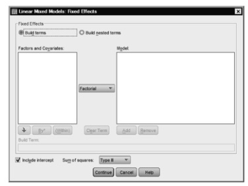
Fig. 12.13. Linear mixed models: Fixed effects.

• Click on Continue, which will take you back to 12.12.
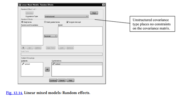
• Click on Random to get 12.14.
• Under Covariance Type, click on the arrow next to Variance Components and scroll down to select Unstructured, which places no constraints on the covariance structure. Whereas in the prior problems, we knew that measurements were likely to be more closely related on adjacent times, we really do not know much about the characteristics of this covariance structure, so we will leave it free to vary.
• Check Include intercept.
• Under Subject Groupings, highlight school and move it into the Combinations: box. Your window should look like 12.14.

• Click on Continue to get back to 12.12.
• Click on Statistics.
• Check Parameter estimates and Tests for covariance parameters. Your window should look like 12.15.

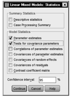
Fig. 12.15. Linear mixed models: Statistics.

• Click Continue.
• Click on OK.

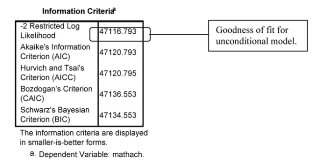
Compare your output and syntax with Output 12.3.

Output 12.3 Unconditional Model of Math Achievement for

Students Nested in Schools

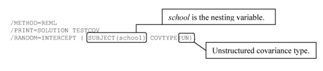
MIXED mathach /CRITERIA=CIN(95) MXITER(100) MXSTEP(5) SCORING(1)

SINGULAR(0.000000000001) HCONVERGE(0, ABSOLUTE) LCONVERGE(0, ABSOLUTE) PCONVERGE(0.000001, ABSOLUTE) /FIXED=| SSTYPE(3)

Mixed Model Analysis

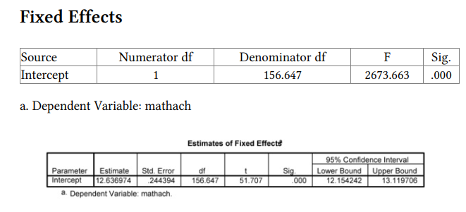
Interpretation of Output 12.3

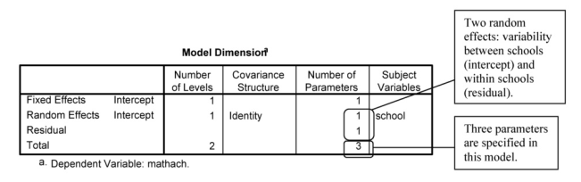
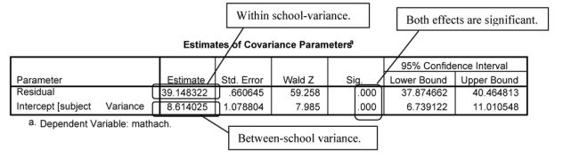
This output is very similar to Output 12.1b, in that it is an unconditional model. This time, there is no repeated-measures variable. Instead, participants are nested in particular schools, which may have their own specific characteristics. The Model dimension table shows that there are 3 parameters. One is the estimate for the fixed intercept effect, which, as before, is not of conceptual interest. The other two are for the random school effect (variability between schools) and residual (variability within schools). The Fixed Effects and Covariance Parameters tables show that all three of these effects are statistically significant (p < .001), showing that the mean is statistically significantly different from zero, and there is significant variability to explain both within schools and between schools. The main purpose of this unconditional model is to see if there is a significant amount of variability in math achievement within schools (the covariance parameter labeled Residual) and variability between schools (the covariance parameter labeled Intercept [subject = Variance school]), and there is. Note that this is the estimate of the variability among the means of the schools.

Example of How to Write About Output 12.3

Results

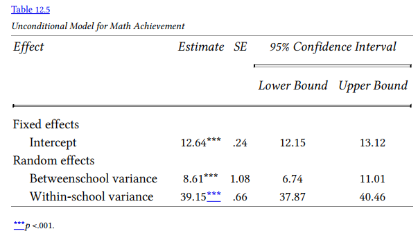
The unconditional repeated-measures model revealed that there was significant variability in the math achievement measure, suggesting that it would be worthwhile to examine a conditional model that could potentially explain some of this variability. (The assumptions of independent observations at the level above the nesting, and random residuals were checked and met. The assumptions of bivariate normality and linear relationships were not met, thus, results should be viewed with caution.) There was statistically significant variability both between schools, Wald Z = 7.99, p < .001 and within schools, Wald Z = 59.26, p < .001. Table 12.5 presents the estimates of the variance components associated with the fixed and random effects.

Source: Leech Nancy L. (2014), IBM SPSS for Intermediate Statistics, Routledge; 5th edition;

download Datasets and Materials.