Application 3: Testing the Factorial Validity of Scores from a Measurement Scale (Second-Order CFA Model) with AMOS

1. Key Concepts

• Model identification issue in higher-order models
• Determination of critical ratio differences
• Specification of equality constraints
• Likert scale scores analyzed as continuous versus categorical data
• Bayesian approach to analyses of categorical data
• Specification and interpretation of diagnostic plots

In contrast to the two previous applications that focused on CFA first-order models, the present application examines a CFA model that comprises a second-order factor. In this chapter, we test hypotheses related to the Chinese version (Chinese Behavioral Sciences Society, 2000) of the Beck Depression Inventory-II (BDI-II; Beck, Steer, & Brown, 1996) as it bears on a community sample of Hong Kong adolescents. The example is taken from a study by Byrne, Stewart, and Lee (2004). Although this particular study was based on an updated version of the original BDI (Beck, Ward, Mendelson, Mock, & Erbaugh, 1961), it nonetheless follows from a series of studies that have tested for the validity of second-order BDI factorial structure for high school adolescents in Canada (Byrne & Baron, 1993, 1994; Byrne, Baron, & Campbell, 1993, 1994), Sweden (Byrne, Baron, Larsson, & Melin, 1995, 1996), and Bulgaria (Byrne, Baron, & Balev, 1996, 1998). The purpose of the ori­ginal Byrne et al. (2004) study was to test the construct validity of a Chinese version of the Beck Depression Inventory (C-BDI-II) for use with Hong Kong community (i.e., nonclinical) adolescents. Based on a randomized tri­adic split of the data (N = 1460), we conducted exploratory factor analysis (EFA) on Group 1 (n = 486), and confirmatory factor analysis (CFA) within the framework of structural equation modeling on Groups 2 (n = 487) and 3 (n = 487); the second CFA served as a cross-validation of the determined factor structure. (For further details regarding the sample, analyses, and results, readers are referred to the original article, Byrne et al., 2004.)

The C-BDI-II is a 21-item scale that measures symptoms related to cognitive, behavioral, affective, and somatic components of depression. Specific to the Byrne et al. (2004) study, only 20 of the 21 C-BDI-II items were used in tapping depressive symptoms for Hong Kong high school adolescents. Item 21, designed to assess changes in sexual interest, was considered to be objectionable by several school principals and the item was subsequently deleted from the inventory. For each item, respondents are presented with four statements rated from 0 to 3 in terms of intensity, and asked to select the one which most accurately describes their own feelings; higher scores represent a more severe level of reported depres­sion. As noted in Chapter 4, the CFA of a measuring instrument is most appropriately conducted with fully developed assessment measures that have demonstrated satisfactory factorial validity. Justification for CFA pro­cedures in the present instance is based on evidence provided by Tanaka and Huba (1984), and replicated in studies by Byrne and colleagues (see above), that BDI score data are most adequately represented by a hierarch­ical factorial structure. That is to say, the first-order factors are explained by some higher-order structure which, in the case of the C-BDI-II and its derivatives, is a single second-order factor of general depression.

Given that each C-BDI (and BDI) item is structured as a Likert 4-point scale, they are considered to represent categorical data and therefore need to be analyzed using estimation methods that can address this issue. Thus, in addition to introducing you to a higher-order CFA model in this chap­ter, I also discuss various issues related to the analysis of categorical data and walk you through the Amos approach to such analyses, which are based on Bayesian statistics. To ease you into the analysis of categorical data based on the Amos Bayesian approach which, in my view, is more difficult than the corrected estimation approach used by other SEM pro­grams, I first work through validation of the C-BDI second-order model with the categorical data treated as if they are of a continuous scale as this is the approach with which you are familiar at this point.

Let’s turn now to a description of the C-BDI-II, and its postulated CFA second-order structure.

2. The Hypothesized Model

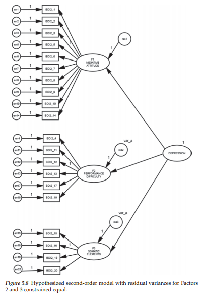
The CFA model to be tested in the present application hypothesizes a priori that (a) responses to the C-BDI-II can be explained by three first-order fac­tors (Negative Attitude, Performance Difficulty, Somatic Elements), and one second-order factor (General Depression); (b) each item has a nonzero load­ing on the first-order factor it was designed to measure, and zero loadings on the other two first-order factors; (c) error terms associated with each item are uncorrelated; and (d) covariation among the three first-order factors is explained fully by their regression on the second-order factor. A diagram­matic representation of this model is presented in Figure 5.1.

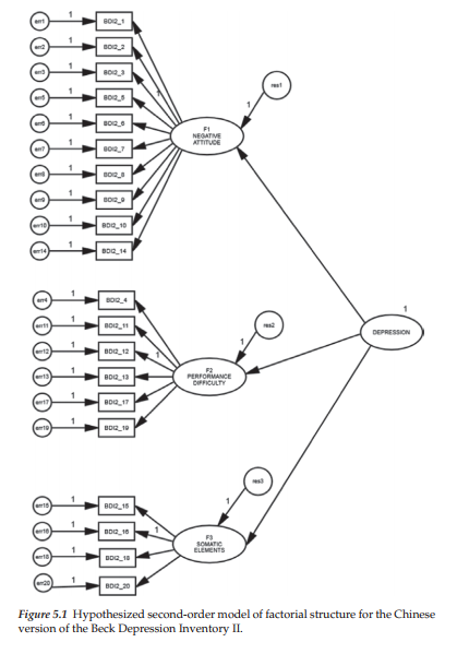
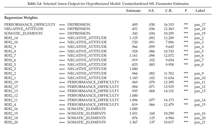
One additional point I need to make concerning this model is that, in contrast to the CFA models examined in Chapters 3 and 4, the factor loading parameter fixed to a value of 1.00 for purposes of model identi­fication here is not the first one of each congeneric group. Rather, these fixed values are specified for the factor loadings associated with BDI2_3 for Factor 1, BDI2_12 for Factor 2 and BDI2_16 for Factor 3. Unfortunately, due to space constraints within the graphical interface of the program, a more precise assignment (i.e., orientation) of these values to their related factor regression paths was not possible. However, these assignments can be verified in a quick perusal of Table 5.6 in which the unstandardized estimates are presented.

3. Modeling with Amos Graphics

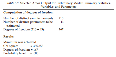
As suggested in previous chapters, in an initial check of the hypothesized model, it is always wise to determine a priori the number of degrees of freedom associated with the model under test in order to ascertain its model identification status. Pertinent to the model shown in Figure 5.1, given 20 items, there are 210 pieces of information contained in the covari­ance matrix ([20 x 21]/2) and 43 parameters to be estimated, leaving 167 degrees of freedom. As noted earlier, Amos provides this information for each model tested (see Table 5.1). Included in the table also is a summary of the number of variables and parameters in the model.

To make sure that you fully comprehend the basis of the related num­bers, I consider it important to detail this information as follows:

Variables (47): 20 observed; 27 unobserved

• Observed variables (20): 20 C-BDI-II items
• Unobserved variables (27): 20 error terms; 3 first-order factors; 1 second-order factor; 3 residual terms
• Exogenous variables (24): 20 error terms; 1 second-order factor; three residual terms
• Endogenous variables (23): 20 observed variables; 3 first-order factors

Parameters

• Fixed
• Weights (26): 20 error term regression paths (fixed to 1.0); 3 factor loadings (fixed to 1.0); 3 residual regression paths (fixed to 1.0)
• Variances: second-order factor
• Unlabeled
• Weights (20): 20 factor loadings
• Variances (23): 20 error variances; 3 residual variances

At first blush, one might feel confident that the specified model is overidentified and, thus, all should go well. However, as noted in Chapter 2, with hierarchical models, it is critical that one also check the identification status of the higher-order portion of the model. In the present case, given the specification of only three first-order factors, the higher-order struc­ture will be just-identified unless a constraint is placed on at least one parameter in this upper level of the model (see e.g., Bentler, 2005; Chen, Sousa, & West, 2005; Rindskopf & Rose, 1988). More specifically, with three first-order factors, we have six ([4 x3]/2) pieces of information; the number of estimable parameters is also six (3 factor loadings; 3 residuals), thereby resulting in a just-identified model. Thus, prior to testing for the validity of the hypothesized structure shown in Figure 5.1, we need first to address this identification issue at the upper level of the model.

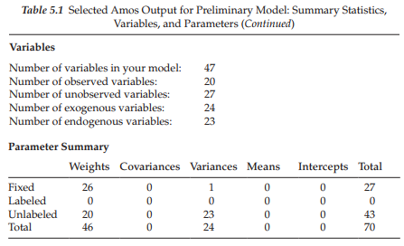
One approach to resolving the issue of just-identification in the present second-order model is to place equality constraints on particular param­eters at the upper level known to yield estimates that are approximately equal. Based on past work with the BDI and BDI-II, this constraint is typ­ically placed on appropriate residual terms. The Amos program provides a powerful and quite unique exploratory mechanism for separating prom­ising, from unlikely parameter candidates for the imposition of equality constraints. This strategy, termed the Critical Ratio Difference (CRDIFF) method, produces a listing of critical ratios for the pairwise differences among all parameter estimates; in our case here, we would seek out these values as they relate to the residuals. A formal explanation of the CRDIFF as presented in the Amos Reference Guide is shown in Figure 5.2. This infor­mation is readily accessed by first clicking on the Help menu and follow­ing these five steps: click on Contents, which will then produce the Search dialog box; in the blank space, type in critical ratio differences; click on List Topics; select Critical Ratios for Diffs (as shown highlighted in Figure 5.2); click on Display. These actions will then yield the explanation presented on the right side of the dialog box.

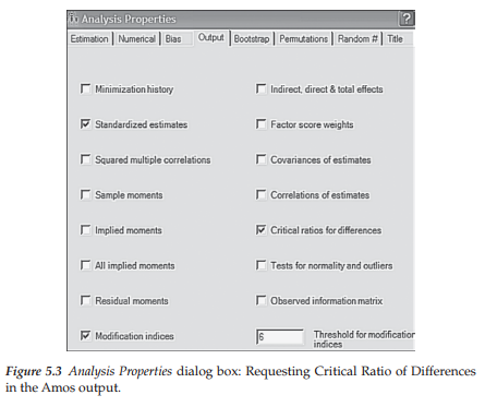
Now that you know how to locate which residual parameters have values that are approximately of the same magnitude, the next step is to know how to obtain these CRDIFF values in the first place. This process, however, is easily accomplished by requesting that critical ratios for differ­ences among parameters be included in the Amos output, which is speci­fied on the Analysis Properties dialog box as shown in Figure 5.3. All that is needed now is to calculate the estimates for this initial model (Figure 5.1). However, at this point, given that we have yet to finalize the identification issue at the upper level of the hypothesized structure, we’ll refer to the model as the preliminary model.

Selected Amos Output File: Preliminary Model

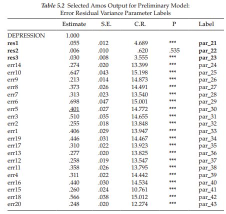
In this initial output file, only labels assigned to the residual parameters and the CRDIFF values are of interest. This labeling action occurs as a con­sequence of having requested the CRDIFF values and, thus, has not been evident on the Amos output related to the models in Chapters 3 and 4. Turning first to the content of Table 5.2, we note that the labels assigned to residuals 1, 2, and 3 are par_21, par_22, and par_23, respectively.

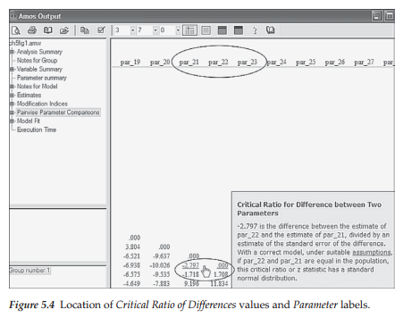
Let’s turn now to the critical ratio differences among parameters, which are shown circled in Figure 5.4. The explanatory box to the bottom right of the circle was triggered by clicking the cursor on the value of -2.797, the CRDIFF value between residl and resid2 (i.e., par_21 and par_22). The boxed area on the upper left of the matrix, as usual, represents labels for the various components of the output file; our focus has been on the “Pairwise Parameter Comparisons” section, which is shown highlighted. Turning again to the residual CRDIFF values, we can see that the two prime candi­dates for the imposition of equality constraints are the higher-order resid­uals related to the Performance Difficulty and Somatic Elements factors as their estimated values are very similar in magnitude (albeit their signs are different) and both are nonsignificant (<1.96). Given these findings, it seems reasonable to constrain variances of the residuals associated with Factors 2 (Performance Difficulty) and 3 (Somatic Elements) to be equal. As such, the higher-order level of the model will be overidentified with one degree of freedom. That is to say, the variance will be estimated for resid2, and then the same value held constant for resid3. The degrees of freedom for the model as a whole should now increase from 167 to 168.

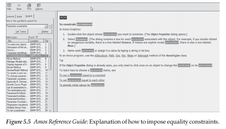
Now that we know which residual terms in the upper level of the model to constrain, we need to include this information in the model to be tested. Such specification of equality constraints in Amos is accomplished by assigning the same label to all parameters being constrained equal. As per all processes conducted in Amos, an elaboration of the specification of equality constraints can be retrieved from the Amos Reference Guide by clicking on the Help tab. The resulting information is shown in Figure 5.5.

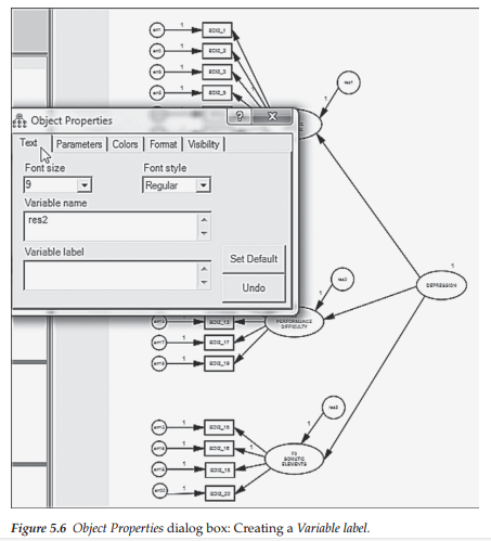
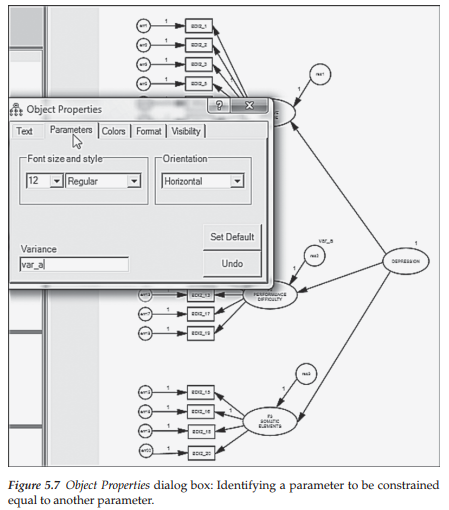
Let’s return, then, to our hypothesized model and assign these equal­ity constraints to the two factor residuals associated with the first-order factors. Turning to the first residual (res2), a right-click on the outside parameter of the circle will open the Tools menu after which we click on the Object Properties tab and the dialog box will likely open with the Text tab selected, where you should see the “Variable name” “res2” already entered as shown in Figure 5.6. Now we want to create a matching label  for this parameter (res2) and for res3 in order that the program will con­sider them to be constrained equal. With the Object Properties tab still open for res2, click on Parameters tab and, in the empty space below marked “Variable label,” insert “var_a” as shown in Figure 5.7. This process is then repeated for the residual term associated with Factor 3 (res3). The fully labeled hypothesized model showing the constraint between these two residual terms is schematically presented in Figure 5.8. Analyses are now based on this respecified model.

Selected Amos Output: The Hypothesized Model

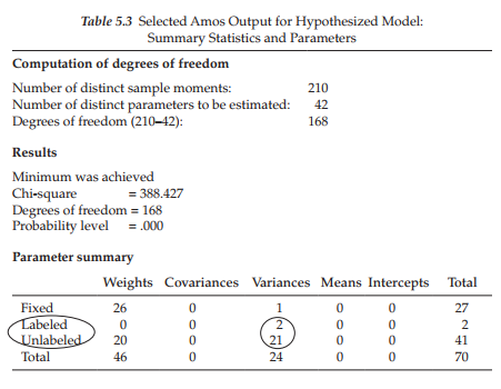
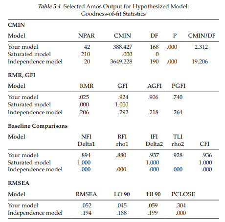
Presented in Table 5.3 is a summary of both the statistics and specified parameters related to the changes made to the original model of C-BDI-II structure. As a consequence of the equality constraints imposed on the model, there are now two important differences from the preliminary model specification. First, as noted earlier, there are now 168, rather than 167 degrees of freedom. Second, there are now two labeled parameters (var_a assigned to both res2 and res3), shown within the ellipsis in Table 5.3.

Model Evaluation

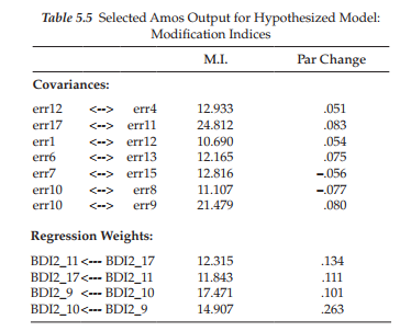
Goodness-of-fit summary. In reviewing the goodness-of-fit statistics in Table 5.4, we can see that the hypothesized model fits the data very well as evidenced by the CFI of .936 and RMSEA of .052. As a consequence we examine the modification indices purely in the interest of completeness. These values are presented in Table 5.5.

Given that MI values less than 10 are conventionally considered to be trivial in SEM, I once again used this value as the default cut point. In reviewing these MIs related to the covariances, you will note two values that are substantially larger than the rest of the estimates. These relate to covariation between the error terms associated with Items 17 and 11 (24.812), and with Items 9 and 10 (21.479). However, as indicated by the reported parameter change statistics, incorporation of these two param­eters into the model would result in parameter values of .083 and .080, respectively—clearly trivial estimates. Turning to the MIs related to regression weights, we see that they make no sense at all as they suggest the impact of one item loading on another. In light of the very good fit of the model, together with the trivial nature of the MIs, we can conclude that the second-order model shown in Figure 5.7 is the most optimal in representing C-BDI-II structure for Hong Kong adolescents.

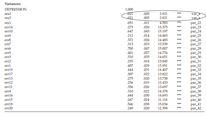
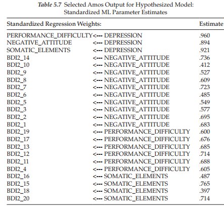
Model ML estimates. As can be seen in Table 5.6, all estimates were found to have critical ratio values >1.96, thereby indicating their statis­tical significance. For clarification regarding terminology associated with the Amos output, recall that the factor loadings are listed as Regression weights. Listed first are the second-order factor loadings followed by the first-order loadings. Note also that all parameters in the model have been assigned a label, which of course is due to our request for the calculation and reporting of CRDIFF values. Turning to the variance estimates, note that all values related to res2 and res3 (encircled) carry exactly the same values, which of course they should. Finally, the related standardized esti­mates are presented in Table 5.7.

In concluding this section of the chapter, I wish to note that, given the same number of estimable parameters, fit statistics related to a model parameterized either as a first-order structure, or as a second-order struc­ture, will basically be equivalent. The difference between the two specifi­cations is that the second-order model is a special case of the first-order model, with the added restriction that structure be imposed on the cor­relational pattern among the first-order factors (Rindskopf & Rose, 1988). However, judgment as to whether or not a measuring instrument should be modeled as a first-order, or as a second-order structure, ultimately rests on the extent to which the first-order factors are correlated, in addition to the substantive meaningfulness as dictated by the underlying theory.

4. Estimation Based on Continous Versus Categorical Data

Thus far in this book, analyses have been based on maximum likelihood (ML) estimation. An important assumption underlying this estimation procedure is that the scale of the observed variables is continuous. In Chapters 3 and 4, as well as the present chapter, however, the observed variables were Likert-scaled items that realistically represent categorical data of an ordinal scale, albeit they have been treated as if they were con­tinuous. Indeed, such practice has been the norm for many years now and applies to frequentist (i.e., traditional, classical) statistical techniques (e.g., AnOVA; MANOVA) as well as SEM analyses. Paralleling this wide­spread practice of treating ordinal data as if they are continuous, however, has been an ongoing debate in the literature concerning the pros and cons of this practice. Given (a) the prevalence of this practice in the SEM field, (b) the importance of acquiring an understanding of the issues involved, and (c) my intent in this chapter to illustrate analysis of data that can address categorically coded variables, I consider it important to address these issues before re-analyzing the hypothesized model of C-BDI-II struc­ture shown in Figure 5.7 via a different estimation approach. First, I pre­sent a brief review of the literature that addresses the issues confronted in analyzing categorical variables as continuous variables. Next, I briefly outline the theoretical underpinning of, the assumptions associated with, and primary estimation approaches to the analysis of categorical varia­bles when such ordinality is taken into account. Finally, I outline the very different approach to these analyses by the Amos program and proceed to walk you through a reanalysis of the hypothesized model previously tested in this chapter.

Categorical Variables Analyzed as Continuous Variables

Prior to perhaps the last 5 years or so, a review of SEM applications reveals most to be based on Likert-type scaled data, albeit with the esti­mation of parameters based on ML procedures. Given the widespread actions of SEM software developers to include more appropriate meth­ods of addressing analyses based on categorical data, there has since been a rapidly growing number of quantitative researchers interested in deter­mining the potential limitations of this practice, as well as the advantages and disadvantages associated with the current alternative estimation strategies (to be described below). We turn now to a brief review of the primary issues. (For a more extensive review of categorical data used within the framework of SEM, see Edwards, Wirth, Houts, & Xi, 2012, and for empirically supported recommendations for treatment of categorical variables as continuous, see Rhemtulla, Brosseau-Laird, & Savalei, 2012.)

The issues. From a review of Monte Carlo studies that have addressed this issue (see, e.g., Babakus, Ferguson, & Joreskog, 1987; Boomsma, 1982; Muthen & Kaplan, 1985), West and colleagues (1995) reported sev­eral important findings. First, Pearson correlation coefficients would appear to be higher when computed between two continuous variables than when computed between the same two variables restructured with an ordered categorical scale. However, the greatest attenuation occurs with variables having fewer than five categories and those exhibiting a high degree of skewness, the latter condition being made worse by vari­ables that are skewed in opposite directions (i.e., one variable positively skewed, the other negatively skewed; see Bollen & Barb, 1981). Second, when categorical variables approximate a normal distribution: (a) The number of categories has little effect on the x² likelihood ratio test of model fit. Nonetheless, increasing skewness, and particularly differential skewness (variables skewed in opposite directions), leads to increasingly inflated x² values. (b) Factor loadings and factor correlations are only modestly underestimated. However, underestimation becomes more crit­ical when there are fewer than three categories, skewness is greater than 1.0, and differential skewness occurs across variables. (c) Error variance estimates, more so than other parameters, appear to be most sensitive to the categorical and skewness issues noted in (b). (d) Standard error esti­mates for all parameters tend to be too low, with this result being more so when the distributions are highly and differentially skewed (see also, Finch et al., 1997).

In summary, the literature to date would appear to support the notion that when the number of categories is large and the data approxi­mate a normal distribution, failure to address the ordinality of the data is likely negligible (Atkinson, 1988; Babakus et al., 1987; Muthen & Kaplan, 1985). Indeed, Bentler and Chou (1987, p. 88) argued that, given nor­mally distributed categorical variables, “continuous methods can be used with little worry when a variable has four or more categories.” More recent findings support these earlier contentions and have further shown that the x² statistic is influenced most by the 2-category response format and becomes less so as the number of categories increases (Green, Akey, Fleming, Hershberger, & Marquis, 1997).

Categorical Variables Analyzed as Categorical Variables

The theory. In addressing the categorical nature of observed variables, the researcher automatically assumes that each has an underlying continuous scale. As such, the categories can be regarded as only crude measurements of an unobserved variable that, in truth, has a continuous scale (Joreskog & Sorbom, 1993) with each pair of thresholds (or initial scale points) represent­ing a portion of the continuous scale. The crudeness of these measurements arises from the splitting of the continuous scale of the construct into a fixed number of ordered categories (DiStefano, 2002). Indeed, this categorization process led O’Brien (1985) to argue that the analysis of Likert-scaled data actually contributes to two types of error: (a) categorization error result­ing from the splitting of the continuous scale into categorical scale, and (b) transformation error resulting from categories of unequal widths.

For purposes of illustration, let’s consider the measuring instrument under study in this current chapter, in which each item is structured on a 4-point scale. I draw from the work of Joreskog and Sorbom (1993), in describing the decomposition of these categorical variables. Let z represent the ordinal variable (the item), and z* the unobserved continu­ous variable. The threshold values can then be conceptualized as follows:

If z* < or = t₁, z is scored 1

If t₁ < z* < or = t₂, z is scored 2

If t₂ < z* < or = t₃, z is scored 3

If t₃ < z*, z is scored 4

where, t₁ < t₂ < t₃ represent threshold values for z*.

In conducting SEM with categorical data, analyses must be based on the correct correlation matrix. Where the correlated variables are both of an ordinal scale, the resulting matrix will comprise polychoric correla­tions; where one variable is of an ordinal scale while the other is of a con­tinuous scale, the resulting matrix will comprise polyserial correlations. If two variables are dichotomous, this special case of a polychoric correl­ation is called a tetrachoric correlation. If a polyserial correlation involves a dichotomous rather than a more general ordinal variable, the polyserial correlation is also called a biserial correlation.

The assumptions. Applications involving the use of categorical data are based on three critically important assumptions: (a) underlying each cat­egorical observed variable is an unobserved latent counterpart, the scale of which is both continuous and normally distributed; (b) sample size is sufficiently large to enable reliable estimation of the related correlation matrix; and (c) the number of observed variables is kept to a minimum. As Bentler (2005) cogently notes, however, it is this very set of assumptions that essentially epitomizes the primary weakness in this methodology. Let’s now take a brief look at why this should be so.

That each categorical variable has an underlying continuous and nor­mally distributed scale is undoubtedly a difficult criterion to meet and, in fact, may be totally unrealistic. For example, in the present chapter, we examine scores tapping aspects of depression for nonclinical adoles­cents. Clearly, we would expect such item scores for normal adolescents to be low, thereby reflecting no incidence of depressive symptoms. As a consequence, we can expect to find evidence of kurtosis, and possibly of skewness, related to these variables, with this pattern being reflected in their presumed underlying continuous distribution. Consequently, in the event that the model under test is deemed to be less than adequate, it may well be that the normality assumption is unreasonable in this instance.

The rationale underlying the latter two assumptions stems from the fact that, in working with categorical variables, analyses must proceed from a frequency table comprising number of thresholds x number of observed variables, to an estimation of the correlation matrix. The prob­lem here lies with the occurrence of cells having zero, or near-zero cases, which can subsequently lead to estimation difficulties (Bentler, 2005). This problem can arise because (a) sample size is small relative to the number of response categories (i.e., specific category scores across all categorical variables; (b) the number of variables is excessively large; and/or (c) the number of thresholds is large. Taken in combination, then, the larger the number of observed variables and/or number of thresholds for these vari­ables, and the smaller the sample size, the greater the chance of having cells comprising zero to near-zero cases.

General analytic strategies. Until recently, two primary approaches to the analysis of categorical data (Joreskog, 1990, 1994; Muthen, 1984) have dominated this area of research. Both methodologies use standard estimates of polychoric and polyserial correlations, followed by a type of asymptotic distribution-free (ADF) methodology for the structured model. Unfortunately, the positive aspects of these categorical variable method­ologies have been offset by the ultra-restrictive assumptions that were noted above and that, for most practical researchers, are both impractical and difficult to meet. In particular, conducting ADF estimation here has the same problem of requiring huge sample sizes as in Browne’s (1984a) ADF method for continuous variables. Attempts to resolve these difficul­ties over the past few years have resulted in the development of several different approaches to modeling categorical data (see, e.g., Bentler, 2005; Coenders, Satorra, & Saris, 1997; Moustaki, 2001; Muthen & Muthen, 1998-2012).

5. The Amos Approach to Analysis of Categorical Variables

The methodological approach to analysis of categorical variables in Amos differs substantially from that of the other programs noted above. In lieu of ML or ADF estimation corrected for the categorical nature of the data, Amos analyses are based on Bayesian estimation. Although Bayesian inference predates frequentist statistics by approximately 150 years (Kaplan & Depaoli, 2013), its application in social/psychological research has been rare. Although this statistical approach is still not widely prac­ticed, Kaplan and Depaoli (2013) have noted a recent growth in its appli­cation which they attribute to the development of updated and powerful statistical software that enables the specification and estimation of SEM models from a Bayesian perspective.

Arbuckle contends that the theoretically correct way to handle ordered-categorical data is to use Bayesian estimation (J. Arbuckle, per­sonal communication, April 2014) and, thus, specification and estima­tion of models based on these types of data using the Amos program are based on this Bayesian perspective. As a follow-up to our earlier test­ing of hypothesized C-BDI-II structure, I now wish to walk you through the process of using this Bayesian estimation method to analyze data with which you are already familiar. As an added bonus, it allows me the opportunity to compare estimated values derived from both the ML and Bayesian approaches to analyses of the same CFA model. I begin with a brief explanation of Bayesian estimation and then follow with a step-by-step walk through each step of the procedure. As with our first application in this chapter, we seek to test for the factorial valid­ity of hypothesized C-BDI-II structure (see Figure 5.7) for Hong Kong adolescents.

What is Bayesian Estimation?

In ML estimation and hypothesis testing, the true values of the model parameters are considered to be fixed but unknown, whereas their estimates (from a given sample) are considered to be random but known (Arbuckle, 2015). In contrast, Bayesian estimation considers any unknown quantity as a random variable and therefore assigns it a probability distribution. Thus, from the Bayesian perspective, true model parameters are unknown and therefore considered to be random. Within this context, then, these parameters are assigned a joint distribution—a prior distribution (prob­ability distribution of the parameters before they are actually observed, also commonly termed the priors; Vogt, 1993), and a posterior distribution (probability distribution of parameters after they have been observed and combined with the prior distribution). This updated joint distribution is based on the formula known as Bayes’s theorem and reflects a combin­ation of prior belief (about the parameter estimates) and empirical evi­dence (Arbuckle, 2015; Bolstad, 2004). Two characteristics of this joint distribution are important to CFA analyses. First, the mean of this pos­terior distribution can be reported as the parameter estimate. Second, the standard deviation of the posterior distribution serves as an analog to the standard error in ML estimation.

Application of Bayesian Estimation

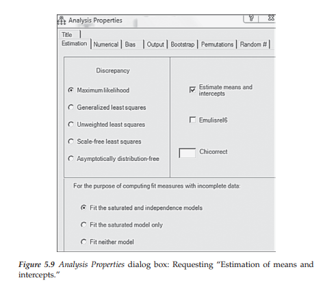
Because Bayesian analyses require the estimation of all observed vari­able means and intercepts, the first step in the process is to request this information via the Analysis Properties dialog box as shown in Figure 5.9. Otherwise in requesting that the analyses be based on this approach you will receive an error message advising you of this fact.

Once you have the appropriately specified model (i.e., the means and intercepts are specified as freely estimated), to begin the Bayesian analyses, click on the S icon in the toolbox. Alternatively, you can pull down the Analyze menu and select Bayesian Estimation. Once you do this, you will be presented with the Bayesian SEM window shown partially in Figure 5.10, and fully in Figure 5.11. Once you request Bayesian estima­tion, the program immediately initiates the steady drawing of random samples based on the joint posterior distribution. This random sampling process is accomplished in Amos via an algorithm termed the Markov Chain Monte Carlo (MCMQ algorithm. Initially, it will appear that noth­ing is happening and you will be presented with a dialog box that reads as “Waiting to accept a transition before beginning burn-in.” Don’t be alarmed as this is not an error message, but merely an advisement that the process has begun. After a brief time lag (3 minutes on my computer), you will observe the numbers in each of the columns to be constantly changing. The reason for these ever-changing numbers is to identify, as closely as possible, the true value of each parameter in the model. This process will continue until you halt the process by clicking on the Pause button, shown within a square frame at the immediate left of the second line of the Toolbox in Figures 5.10 and 5.11.

Now, let’s take a closer look at the numbers appearing in the upper section (the Toolbox) of the Bayesian SEM window. In Figure 5.10, note the numbers beside the Pause button, which read as 500 + 65.501 and indicate the point at which sampling was halted. This information conveys the infor­mation that Amos generated and discarded 500 burn-in samples (the default value) prior to drawing the first one that was retained for the analysis. The reason for these burn-in samples is to allow the MCMC procedure to con­verge to the true joint posterior distribution (Arbuckle, 2015). After draw­ing and discarding the burn-in samples, the program then draws additional samples, the purpose of which is to provide the most precise picture of the values comprising the posterior distribution. At this pause point, the num­bers to the right of the “+” sign indicate that the program has randomly drawn 65.501 samples (over and above the 500 burn-in samples).

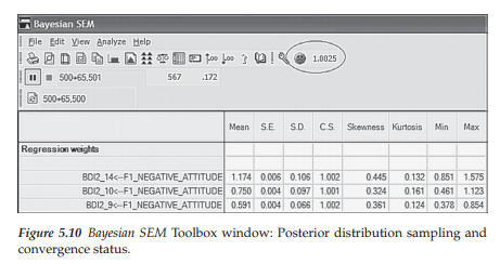
Clearly, a logical question that you might ask about this sampling pro­cess is how one knows when enough samples have been drawn to yield a posterior distribution that is sufficiently accurate. This question addresses the issue of convergence and the point at which enough samples have been drawn so as to generate stable parameter estimates. Amos establishes this cutpoint on the basis of the Convergence Statistic (CS), which derives from the work of Gelman, Carlin, Stern, & Rubin (2004). By default, Amos consid­ers the sampling to have converged when the largest of the CS values is less than 1.002 (Arbuckle, 2015). The last icon on the upper part of the output rep­resents the Convergence Statistic. Anytime the default CS value has not been reached, Amos displays an unhappy face (©). Turning again to Figure 5.10, I draw your attention to the circled information in the Toolbar section of the window. Here you will note the unhappy face accompanied by the value of 1.0025, indicating that the sampling process has not yet attained the default cutpoint of 1.002; rather, it is ever so slightly higher than that value.

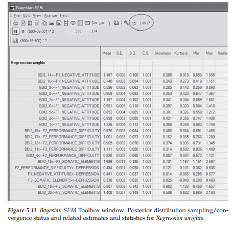
In contrast, turn now to Figure 5.11 in which you will find a happy face (0)¹ together with the CS value of 1.0017, thereby indicating conver­gence (in accordance with the Amos default value). Moving down to the row that begins with the Pause icon, we see the numbers 500 + 59.501. This information indicates that following the sampling and discarding of 500 burn-in samples, the MCMC algorithm has generated 59 add­itional samples and, as noted above, reached a convergent CS value of 1.0017.

Listed below the toolbar area are the resulting statistics pertinent to the model parameters; only the regression weights (i.e., factor loadings) are presented here. Each row in this section describes the posterior dis­tribution value of a single parameter, while each column lists the related statistic. For example, in the first column (labeled Mean), each entry repre­sents the average value of the posterior distribution and, as noted earlier, can be interpreted as the final parameter estimate. More specifically, these values represent the Bayesian point estimates of the parameters based on the data and the prior distribution. Arbuckle (2015) notes that with large sample sizes, these mean values will be close to the ML estimates. (This comparison is illustrated later in the chapter.)

The second column, labeled “S.E.”, reports an estimated standard error that implies how far the estimated posterior mean may lie from the true posterior mean. As the MCMC procedure continues to generate more samples, the estimate of the posterior mean becomes more accurate and the S.E. will gradually drop. Certainly, in Figure 5.11, we can see that the S.E. values are very small, indicating that they are very close to the true values. The next column, labeled S.D., can be interpreted as the likely dis­tance between the posterior mean and the unknown true parameter; this number is analogous to the standard error in ML estimation. The remain­ing columns, as can be observed in Figure 5.11, represent the posterior distribution values related to the CS, skewness, kurtosis, minimum value, and maximum values, respectively.

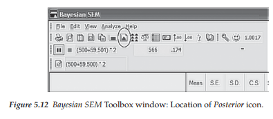
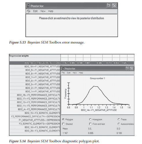
In addition to the CS value, Amos makes several diagnostic plots avail­able for you to check the convergence of the MCMC sampling method. To generate these plots, you need to click on the Posterior icon located in the Bayesian SEM Toolbox area, as shown encased in an ellipse in Figure 5.12. However, it is necessary first to identify the parameter for which you are requesting graphical information, as failure to select a parameter will gen­erate the dialog box shown in Figure 5.13. As can be seen highlighted in Figure 5.14, I selected the first model parameter, which represents the load­ing of C-BDI-II Item 14 onto Negative Attitude (Factor 1). Right-clicking the mouse generated the Posterior Diagnostic dialog box with the distri­bution shown within the framework of a polygon plot. Specifically, this frequency polygon displays the sampling distribution of Item 14 across 59 samples (the number sampled after the 500 burn-in samples were deleted).

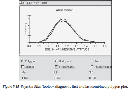
Amos produces an additional polygon plot that enables you to deter­mine the likelihood that the MCMC samples have converged to the poster­ior distribution via a simultaneous distribution based on the first and last thirds of the accumulated samples. This polygon is accessed by selecting “First and last” as can be seen in Figure 5.15. From the display in this plot, we observe that the two distributions are almost identical, suggesting that Amos has successfully identified important features of the posterior dis­tribution of Item 14. Notice that this posterior distribution appears to be centered at some value near 1.7, which is consistent with the mean value of 1.167 noted in Figure 5.11.

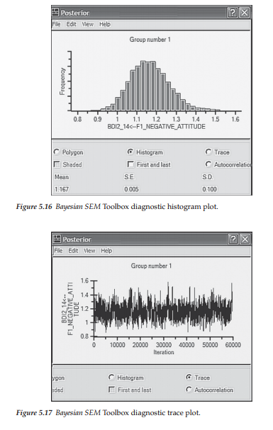
Two other available diagnostic plots are the histogram and trace plots illustrated in Figures 5.16 and 5.17 respectively. While the histogram is rela­tively self-explanatory, the trace plot requires some explanation. Sometimes termed the time-series plot, this diagnostic plot helps you to evaluate how quickly the MCMC sampling procedure converged in the posterior distri­bution. The plot shown in Figure 5.17 is considered to be very good as it exhibits rapid up-and-down variation with no long-term trends. Another way of looking at this plot is to imagine breaking up the distribution into sections. Results would show none of the sections to deviate much from the rest. This finding indicates that the convergence in distribution occurred rapidly, a clear indicator that the SEM model was specified correctly.

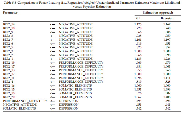
As one final analysis of the C-BDI-II, let’s compare the unstandard­ized factor loading estimates for the ML method versus the Bayesian posterior distribution estimates. A listing of both sets of estimates is pre­sented in Table 5.8. As might be expected, based on our review of the diag­nostic plots, these estimates are very close relative to both the first- and second-factor loadings. These findings speak well for the validity of our hypothesized structure of the C-BDI for Hong Kong adolescents.

I wish to underscore the importance of our comparative analysis of C-BDI-II factorial structure from two perspectives: ML and Bayesian estimation. Given that items comprising this instrument are based on a 4-point scale, the argument could be made that analyses should be based on a methodology that takes this ordinality into account. As noted earlier in this chapter, historically these analyses have been based on ML meth­odology, which assumes the data are of a continuous scale. Importantly, however, I also reviewed the literature with respect to (a) why research­ers have tended to treat categorical variables as if they are continuous in SEM analyses, (b) the consequence of treating categorical variables as if they are of a continuous scale, and (c) identified scaling and other statis­tical features of the data that make it critical that the ordinality of categor­ical variables be taken into account, as well as conditions that show this approach not to make much difference. At the very least, the researcher always has the freedom to conduct analyses based on both methodological approaches and then follow up with a comparison of the parameter esti­mates. In most cases, where the hypothesized model is well specified and the scaling based on more than five categories, it seems unlikely that there will be much difference between the findings.

In the interest of space, this overview of analysis of a CFA model using a Bayesian approach has necessarily been brief and focused solely on its application in the testing of categorical data as implemented in the Amos program. However, for a very easy-to-read and largely nonmathemati­cal overview of how this Bayesian approach is used and applied in SEM, together with its theoretical and practical advantages, readers are referred to van de Schoot et al. (2014).

One final comment regarding analysis of categorical data in Amos relates to its alphanumeric capabilities. Although our analyses in this chapter were based on numerically-scored data, the program can just as easily analyze categorical data based on a letter code. For details regard­ing this approach to SEM analyses of categorical data, as well as many more details related to the Bayesian statistical capabilities of Amos, read­ers are referred to the user’s manual (Arbuckle, 2015).

6. Modeling with Amos Tables View

In closing out this chapter, let’s now review specification of our second-order C-BDI-II model (see Figure 5.1) as replicated in Tables View format and partially portrayed in Figure 5.18. Once again, the reason for the partial reproduction of this tabled form of the specified model is due to its length pertinent to both the Variables and Regression weights. Given that the specification is of a second-order model, of course, there is no Covariance section here.

In retrieving the equivalent Tables View version of the hypothesized model shown in Figure 5.1, I was surprised to find that the presentation of the entries for both the Variables and Regression weights sections were badly misplaced in several places. Unfortunately, despite several attempts to rectify this misplacement problem, I was unable to do so. In checking on this mismatched presentation of the specified model, I was subsequently advised that reorientation of this information is not possible for the Tables View spreadsheet (J. Arbuckle, personal communication, December 11, 2014). However, rest assured that all parameters are definitely included in the Tables View spreadsheet; I just want to caution you that in viewing them on your computer, you will quickly see that some are listed in what I con­sider to be a displaced position. For example, on Figure 5.18, which pro­vides only a partial showing of the specification list, note the location of the entry for BDI2_18 and its accompanying error term (err18). For consistency with the other regression weights, this row more appropriately should have been inserted after the entry for BDI2_18 and its accompanying column that includes the entry “F3 SOMATIC ELEMENTS.” Still another example in the shortened list is the mismatched listing of the three first-order latent factors. This problem of misplacement, I suspect, likely arises from the fact that the model of interest here is a second-order model, which entails a slightly more complex format than the previous models in Chapters 3 and 4.

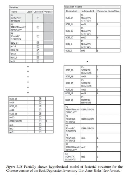
As with the previous chapters, a review of the necessarily reduced Variables table on the left side of the figure is very straightforward in show­ing all checked cells to represent all items (i.e., the observed variables). In addition to the BDI2 items, there is also a listing of the higher-order latent factor of Depression, together with its three related residuals. Recall that the variance of this higher-order factor was fixed to 1.00, which is indicated in the Variance column. In contrast, the three residuals represent latent variables with their variances to be estimated.

Turing to the Regression weights table, you will observe that the regres­sion path of all error terms related to each of the six items included in Figure 5.18 has been fixed to a value of 1.0, in addition to the regression path (i.e., factor loading) of item BDI2_16 as indicated in the Parameter Name/ Value column. These constraints, of course, are consistent with the path dia­gram of the model tested (see Figure 5.1). Of further mention, as indicated by the subtitles, all items are listed as Dependent variables, whereas all latent variables (factors and error terms) are listed as Independent variables.

Appearing in the same block, but following the first part of this block, are the listing of the three first-order factors as Dependent variables along with the second-order factor of Depression as Independent variables. Finally, the last three rows once again list the first-order factors as Dependent variables accompanied by the residuals listed in the second column as Independent variables, with each residual indicated as having its regression path fixed to a value of 1.0, which again can be seen in Figure 5.1.

Source: Byrne Barbara M. (2016), Structural Equation Modeling with Amos: Basic Concepts, Applications, and Programming, Routledge; 3rd edition.