Categorical Moderators in meta-analysis

1. Evaluating the Significance of a categorical Moderator

The logic of evaluating categorical moderators in meta-analysis parallels the use of ANOVA in primary data analysis. Whereas ANOVA partitions variability in scores across individuals (or other units of analysis) into variability existing between and within groups, categorical moderator analysis in meta-analysis partitions between-study heterogeneity into that between and within groups of studies (Hedges, 1982; Lipsey & Wilson, 2001, pp. 120-121). In other words, testing categorical moderators in meta-analysis involves comparing groups of studies classified by their status on some categorical moderator.

Given this logic of partitioning heterogeneity, it makes sense to start with the heterogeneity equation (Equation 8.6) from Chapter 8, reproduced here for convenience:

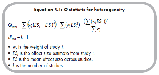
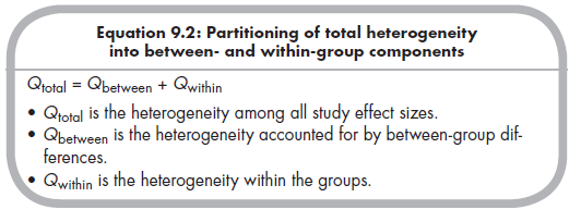
You might have noticed that I have changed the notation of this equation slightly, now giving the subscript “total” to this Q statistic. The reason for this subscript is to make it explicit that this is the total, overall heterogeneity among all effect sizes. The logic of testing categorical moderators is based on the ability to separate this total heterogeneity (Qtotal) into two components, the between-group heterogeneity (Qbetween) and the within-group heteroge­neity (Qwithin), such that:

The key question when evaluating categorical moderators is whether there is greater-than-expectable between-group heterogeneity. If there is, then this implies that the groups based on the categorical study character­istic differ and that the categorical moderator is therefore reliably related to effect sizes found in the studies. If the groups do not differ, then this implies that the categorical moderator is not related to effect sizes (or, in the language of null hypothesis significance testing, that you have failed to find evidence for this moderation).

The most straightforward way to compute the between-group heterogene­^ity ⁽Qbetween^{) is to rearran}g^e Eq^uati°ⁿ 9.^{2, s}° ^that Qbetween = Qtotal ^– Qwithin. Because you have already computed the total heterogeneity (Qt_otali Equation 9.1), you only need to compute and subtract the within-group heterogeneity (Q_withi_n) to obtain the desired Qb_et_ween. To compute the heterogeneity within each group, you apply a formula similar to that for total heterogeneity to just the studies in that group:

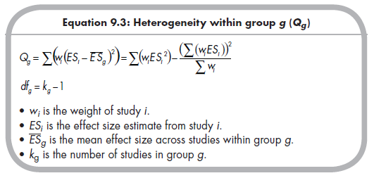
That is, you compute the heterogeneity within each group (g) using the same equation as for computing total heterogeneity, restricting the included studies to only those studies within group g. After computing the within-group heterogeneity (Qg) for each of the groups, you compute the within-group heterogeneity (Q_withi_n) simply by summing the heterogeneities (Qgs) from all groups. More formally:

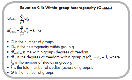
As mentioned, after computing the total heterogeneity (Qtotal) and the within-group heterogeneity (Qwithin), you compute the between-group heterogeneity by subtracting the within-group heterogeneity from the total heterogeneity (i.e., Qbetween = Qtotal – Qwithin; see Equation 9.2). The statistical significance of this between-group heterogeneity is evaluated by considering the value of Qbetween relative to dfbetween, with dfbetween = G – 1. Under the null hypothesis, Qbetween is distributed as c2 with dfbetween, so you can consult a chi-square table (such as Table 8.2; or use functions such as Microsoft Excel’s “chiinv” as described in footnote 6 of Chapter 8) to evaluate the statistical significance to make inferences about moderation.

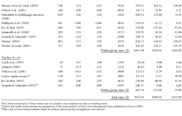
To illustrate this test of categorical moderators, consider again the exam­ple meta-analysis of 22 studies reporting associations between children and adolescents’ relational aggression and rejection by peers. As shown in Chap­ter 8, these studies yield a mean effect size Z_r = .387 (r = .368), but there was significant heterogeneity among these studies around this mean effect size, Q(21) = 291.17, p < .001. This heterogeneity might suggest the importance of explaining this heterogeneity through moderator analysis, and I hypothe­ sized that one source of this heterogeneity might be due to the use of different reporters to assess relational aggression. As shown in Table 9.1, these studies variously used observations, parent reports, peer reports, and teacher reports to assess relational aggression, and this test of moderation evaluates whether associations between relational aggression and rejection systematically differ across these four methods of assessing aggression.

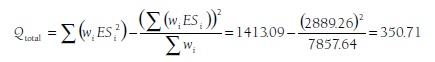
I have arranged these 27 effect sizes (note that these come from 22 inde­pendent studies; I am using effect sizes involving different methods from the same study as separate effect sizes¹) into four groups based on the method of assessing aggression. To compute Q_total, I use the three sums across all 27 studies (shown at the bottom of Table 9.1) within Equation 9.1:

I then compute the heterogeneity within each of the groups using the sums from each group within Equation 9.3. For the three observational stud­ies, this within-group heterogeneity is

Using the same equation, I also compute within-group heterogeneities of Qwithin_parent = 0.00 (there is no heterogeneity in a group of one study), Qwithin_teacher = 243.16, and Qwithin_teacher = 40.73. Summing these values yields Qwithin = 1.68 + 0.00 + 243.16 + 40.73 = 285.57. Given that Qbetween = Qtotal – Q_withi_n, the between-group heterogeneity is Qb_et_ween = 350.71 – 285.57 = 65.14. This Qbetween is distributed as chi-square with df = G – 1 = 4 – 1 = 3 under the null hypothesis of no moderation (i.e., no larger-than-expected between group differences). The value of Qbetween in this example is large enough (p < .001; see Table 8.2 or any chi-square table) that I can reject this null hypothesis and accept the alternate hypothesis that the groups differ in their effect sizes. In other words, moderator analysis of the effect sizes in Table 9.1 indicates that method of assessing aggression moderates the asso­ciation between relational aggression and peer rejection.

2. Follow-Up Analyses to a Categorical Moderator

If you are evaluating a categorical moderator consisting of two levels—in other words, a dichotomous moderator variable—then interpretation is simple. Here, you just conclude whether the between-group heterogeneity
is significant, then inspect the within-group mean effect sizes (i.e., weighted means computed using studies from each group separately). The decision and interpretation is then straightforward as to which group of studies yields stronger effect sizes.

The situation is more complex when the categorical moderator has three or more levels—that is, when the moderator test is an omnibus compari­son. Here, the significant between-group heterogeneity indicates that at least some groups differ from others, but exactly where those differences lie is unclear. This situation is akin to follow-up analyses conducted with a three or more level ANOVA, and decisions of how to handle these situations in meta-analysis are as thorny as they are for ANOVAs used in primary studies. However, the variety of possibilities that exist for ANOVA follow-up analyses have not been translated into a meta-analytic framework. Therefore, the two choices are between an overly liberal and an overly conservative approach.

2.1. The Liberal Approach

This approach is liberal in that one makes no attempt to control cumulative (a.k.a. family-wise) type I errors when following up a finding of significant between-group heterogeneity. Instead, you just perform a series of all pos­sible two-group comparisons to identify which groups differ in the magni­tudes of their effect sizes. To perform these comparisons, you would use the same logic described in the previous subsection for testing between-group heterogeneity, but would (1) restrict the calculation of total heterogeneity (Qtotal) to studies from the two groups, (2) sum the within-group heteroge­neity (Q_within) only from these two groups, and (3) evaluate the resultant between-group heterogeneity (Q_between) as a 1 df c² test (because G = 2 in this comparison, so dƒ_between = 2 – 1). You would then repeat this two-group comparison for all possible combinations among the groups of the categorical moderator (the total number of comparisons is G(G-1)/2).

This approach parallels Fisher’s Least Significant Difference test in ANOVA (see e.g., Keppel, 1991, p. 171). Like this test in ANOVA, the obvi­ous problem with using this approach in categorical moderator analyses in ANOVA is that it allows for higher-than-desired rates of type I error in the follow-up comparisons (i.e., not controlling for cumulative, or family-wise, type I error). A second problem with this approach occurs when different groups have different effective sample sizes (i.e., many studies with large samples vs. few studies with small samples) or amounts of within-group het­erogeneity. In these situations, this approach can yield surprising results, in which groups that appear to have quite different average effect sizes are not found to differ (because the groups have small effective sample sizes or large heterogeneity), whereas groups that seem to have more similar average effect sizes are found to differ (because the groups have large effective sample sizes or small heterogeneity).

2.2. The Conservative Approach

A conservative approach to multiple follow-up comparisons of a significant omnibus moderator result parallels the approach in ANOVA commonly called Bonferroni correction (a.k.a. Dunn test; see Keppel, 1991, p. 167). Using this approach, you make the same series of comparisons between all possible two- group combinations as in the liberal approach, but the resultant Qb_et_weens are evaluated using an adjusted level of statistical significance (i.e., some value smaller than the chosen type I error rate, e.g., a = .05). Specifically, you divide the desired type I error rate (e.g., a = .05) by the number of comparisons² made (i.e., by G(G – 1)/2). This Bonferroni-adjusted level of significance (ag) is then used as the basis for making inferences about whether the between- group heterogeneity statistics (Qb_et_ween) provide evidence to reject the null hypotheses (i.e., concluding that groups differ).

There are two limitations to this approach. First, like this approach used in ANOVAs in primary studies, it is overly conservative and leads to diminished statistical power (i.e., higher type II error rates). The extent to which this limitation is problematic will depend on the sample sizes and numbers of studies in the groups you wish to compare. If all groups of the categorical moderator contain a large number of studies with large sample sizes (i.e., there is high statistical power), then the cost of this overly conser­vative approach might be minimal. However, if even some of the groups have a small number of studies or small sample sizes, then the loss of statistical power is problematic. The second limitation of this conservative approach is similar to that of the liberal approach—that seemingly larger differences in group mean effect sizes might not be significantly different, whereas seem­ingly small differences are found to be different.

2.3. Conclusions Regarding Follow-Up Analyses

The choice between an overly liberal and an overly conservative approach is not an easy one to make. In weighing between these approaches, I sug­gest that you consider (1) the relative cost of type I (erroneously concluding differences) versus type II (failing to detect differences) errors, and (2) the expectable power of your meta-analysis (meta-analyses with many studies with large sample sizes tend to have high power). Alternatively, you might avoid this problem by specifying meaningful planned contrasts that can be evaluated within a regression framework (see below).

Source: Card Noel A. (2015), Applied Meta-Analysis for Social Science Research, The Guilford Press; Annotated edition.