An Alternative SEM Approach for Moderation in meta-analysis

Cheung (2008) described an approach to meta-analysis within an SEM frame­work that can be used for moderator analyses as described in this chapter, as well as estimating fixed-effects means as described in Chapter 8 and more complex models (random- and mixed-effects models) described in Chapter 10. You should be aware that this is not SEM in the sense of multivariate, latent variable analyses (such as described in Chapter 12), but instead uses the flexibility of the SEM approach and software (e.g., ability to place model constraints) to fit meta-analytic models of a single effect size and coded study characteristics as predictors. In the context of moderator analyses, this approach is also advantageous over the regression approach I have described earlier in that it can use the advanced methods of missing data management in SEM when some studies do not report values for the characteristics you wish to evaluate as moderators.⁸

Although this alternative SEM approach is flexible, it does require an understanding of SEM as well as the use of specialized software.⁹ Given this restriction, I will write this section with the assumption that you are familiar with SEM (if you are not, I recommend Kline, 2010, as an accessible introduc­tion). Next, I describe the data transformation central to this approach, how this model can be used to estimate (fixed-effects) mean effect sizes (Chapter 8), and how this model can be used for moderator analyses. I consider this model again in Chapter 10 when I describe how it can be used for random- and mixed-effects models.

1. Transformations to Produce Equal Errors across Studies

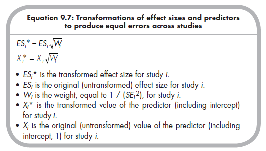
As you recall, different studies in a meta-analysis are believed to have differ­ent sampling variances (i.e., squared standard errors) that provided the basis for differentially weighting the studies (see Chapter 8). The initial “key” to this SEM approach to meta-analysis is to rescale effect sizes and their predic­tors for each study so that the studies have equal sampling errors. This allows you to treat each study as an equally weighted case in the analyses because the weighting is accounted for by a transformation of study effect sizes and their predictors (i.e., study characteristics). This transformation factor is the square root of the weight you would normally use for a fixed-effects analysis (i.e., Wj = 1 / SE;²). You apply this transformation factor by multiplying it by the effect sizes and predictors (including the intercept) (Cheung, 2008,186):

Once these transformed effect sizes and predictors are created, the anal­yses within an SEM context do not require additional weighting, so each study is treated as an equally weighted case (to be clear, studies are still dif­ferentially weighted, but this occurs in the transformation rather than in the analyses). Next, I describe and illustrate how this approach can be used to estimate (fixed-effects) mean effect sizes and to evaluate moderators. This presentation follows closely that of Cheung (2008), but I use the example meta-analysis of relational aggression and peer rejection to illustrate these analyses.

2. Estimating Mean Effect Sizes

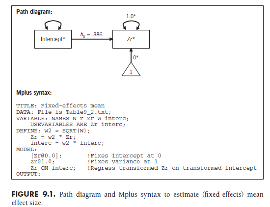
Although you already know how to estimate mean effect sizes (Chapter 8), it is useful to revisit these issues within this SEM approach. To evaluate a mean effect size, a model is fit in which the transformed effect size (ES*) is regressed onto the transformed intercept (Xq*). The intercept is just a con­stant 1.0 (literally, a variable with the value of 1 for each study) that is then transformed using Equation 9.7. Although the model is simple and could otherwise be performed using traditional software for regression, there are two important constraints you need to place on this model that require SEM software: (1) you fix the variance of ES* to 1.0, and (2) you fix the indicator intercept of ES* to 0. Given these constraints, the mean effect size is repre­sented as the regression coefficient from the transformed intercept.

I demonstrate this SEM representation by estimating the mean of the relational aggression with rejection association among the 22 studies shown in Table 9.2. To illustrate the computations of Equation 9.7, consider the first study (Blachman, 2003), which had an effect size Z_r = .583 and weight (W) = 208.12. Using Equation 9.7, I find that the transformed effect size, Z_r*, is equal to .583V208.12 = 8.411. The predictor in this model is a transformed intercept 1.0, computed using Equation 9.7 to be W208.12 = 14.426. I also apply these transformations of effect sizes and intercept to the other 21 stud­ies in Table 9.2.

The path diagram representing this analysis, as well as Mplus syntax,¹⁰ is shown in Figure 9.1. From this figure, you see that the transformed effect size (Fisher’s Z_r, subjected to the transformation of Equation 9.7 to obtain Z_r*) is regressed onto the transformed intercept (the constant 1.0 transformed with Equation 9.7 to obtain X*). The regression coefficient (bo) in this example is estimated to be .386, which is identical (within rounding error) to the mean Z_r from these studies using the methods I described in Chapter 8. The standard error of this estimate is .012, which is also identical to the standard error of the mean effect size computed in Chapter 8. Therefore, the statistical significance (Z = .386/012 = 32.68, p < .001) is also identical (within round­ing) to the previously obtained results. In short, this approach yields identi­cal values to those if you used the methods described in Chapter 8.

3. Evaluating Moderators

From here, it is straightforward to add predictors to evaluate (categorical or continuous) moderators of this effect size. You simply make the same trans­formation described in Equation 9.7 (i.e., multiplying by the square root of the weight) to these predictors, and then add them to the predictive model.

I illustrate this analysis using the meta-analysis summarized in Table 9.3, in which I want to evaluate age (a continuous variable) and method of measuring aggression (three dummy coded variables) as potential modera­tors of the relational aggression with peer rejection association. As I did ear­lier using the multiple regression approach, I center these variables to assist interpretation.

Considering the first study, the effect size and intercept are transformed as already described. For this study, the centered values of the moderators (i.e., the values of Table 9.3 minus their means) are C_Age = -0.33 (= 9.2 – 9.53), EC1 = 0.97 (= 1 – .03), EC2 = -0.82, and EC3 = -0.12. When these four predictors are transformed (Equation 9.7) by multiplying by the square root of the study weight, the transformed values are C_Age* = -4.76, EC1* = 13.99, EC2* = -11.83, and EC3* = -1.73.

Figure 9.2 shows the path diagram and Mplus script for adding cen­tered age and the three effects codes representing measurement type, to evaluate these coded study characteristics as moderators of the association between relational aggression and rejection. You evaluate moderator effects by inspecting the regression coefficients of the transformed moderators pre­dicting transformed effect size. In this example, as when performed within a regression context, each of the three effects codes (EC1: b1 = 0.582, SE = .092, Z = 6.30, p < .001; EC2: b₂ = 0.415, SE = .063, Z = 6.55, p < .001; EC3: b₃ = 0.152, SE = .068, Z = 2.24, p < .05) as well as centered age (b4 = -0.020, SE = .004, Z = 5.33, p < .001) were significant moderators. Further, the intercept was significant and represents the overall mean Z_r (bg = 0.370, SE = .011, Z = 32.78, p < .001). All of these values are identical (within rounding error) to those found through regression analyses. However, the key advantage of this SEM approach is that it could have accommodated all studies even if some had missing values for the study characteristics age or method of assessing aggression.

Source: Card Noel A. (2015), Applied Meta-Analysis for Social Science Research, The Guilford Press; Annotated edition.