CFA Example in AMOS

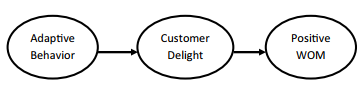
Let’s say I want to test a simple model that has three unobserved variables. The first vari- able is a concept called “Adaptive Behavior”, which explores customer’s perceptions that an employee adapted their behavior to the customer during an experience. This adaptation could be through verbal interaction or through their direct actions. The perceived Adap- tive Behavior construct is hypothesized to positively influence feelings of Customer Delight, which is going to influence intentions to spread positive word of mouth about the experience (Positive WOM).

The construct of Adaptive Behavior has 5 indicators, and the other two constructs have 3 indicators each. Once I have collected and screened my data, I am ready to perform a CFA. The first thing you need to do is to read in your data file to AMOS (I have listed the data file as Customer Delight Data).You need to select the “Data Files”  icon.The following window will appear:

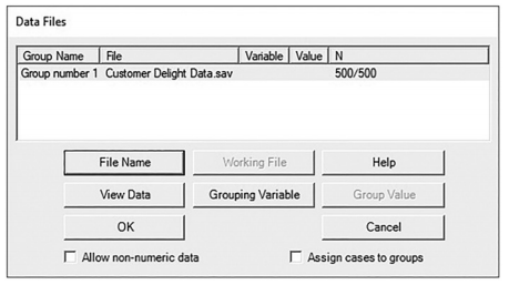
Figure 4.4 Data Files Pop-Up Window

Click on “File Name”, find your data file, and then hit OK.You should also see the number of responses in the data file (N). Next, you need to click the variable icon:

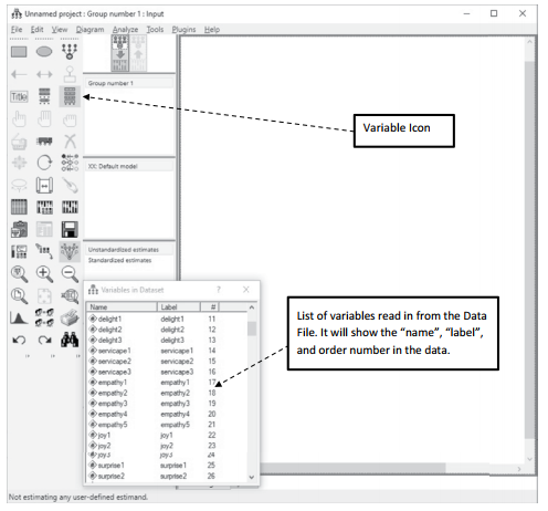
Figure 4.5 List of Variables AMOS Window

You will then draw out your unobservable variables along with denoting the indicators for each construct. Remember, the “Draw Latent Variable” icon is the easiest way to do this . After selecting this icon, drag your circle (indicating the unobservable) to the desired size, then click in the circle to add the number of indicators. If you click in the circle three times, it will add three indicators. If you forget to add enough indicators, no problem; just make sure the “Draw Latent Variable” icon is selected and then click in the circle again to add another indicator. Once you form the unobserved variable and indicators, you will then drag in from the variable window your measured items to the indicator boxes for the specific construct.You will also need to label your unobserved constructs.You can let AMOS do it for you, but I do not suggest this. To label the unobserved construct, you need to right-click on the unobserved variable you want to label. Next, you need to select “Object Properties” (you can also double click into a variable and it will bring up object properties). In the variable name section, you will label your construct. Please note that all variable names for your constructs and indicators must be unique.You cannot have the same name for multiple things in your model, or AMOS will not be able to clearly run the analysis and will ultimately give you an error message.You cannot have spaces between words in a variable name; AMOS will recognize the space as an illegal character and stop the analysis. I typically use the underscore character to denote a space between words. After dragging in your indicators from the vari- able view and labeling your unobserved constructs, you might need to select the “Change Shape” icon .This will let you change the size of your circles or squares of your variables to see the full name of each one listed. You will also notice that with each indicator added, AMOS will automatically include an error term for that indicator. Every error term has to be labeled as well. This can be a painstaking process if you have a lot of indicators. As noted in the “Tips” section in Chapter 3, AMOS has a function that will label all the error terms for you.

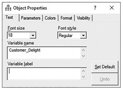
Figure 4.6 Object Properties Pop-Up Window

A few things need to be addressed about AMOS before we move on. First, you will notice that AMOS automatically sets the metric with one of your indicators (constrained to 1.0), so that you do not have to do that. If you decide for whatever reason to delete that indicator, you will need to set the metric on another indicator. This can be done by double clicking on another indicator arrow which will bring up the “Object Properties window”.You will then need to select the “Parameters” tab at the top of the pop-up window, and then place a “1” in the “Regression Weight” field. Second, all unobserved constructs in a CFA are considered independent constructs, which means a covariance needs to be added between every con- struct. In small models with a few constructs, it is just easier to select the “Draw Covari- ance” button and connect the constructs one at a time. If you have a very large number of constructs, then see the “Tips” section in Chapter 3 on how to covary multiple independent constructs at once. Lastly, AMOS will require you to save and label the project you are work- ing on before an analysis will take place.You would be well served to save your file names that list the specific analysis and subject of the project.

To see the completed graphical diagram of the CFA for our three construct model, see Figure 4.7.

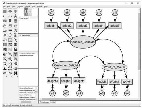
Figure 4.7 Three Construct CFA Model in AMOS

Before you run the CFA analysis, you need to select the “Analysis Properties” icon . This will start a pop-up window that will ask how much detail you want in the output of the analysis. Go to the “Output” tab at the top of the pop-up window, which will give all the pos-sible options. I prefer to select “Minimization History, Standardized Estimates, and Square Multiple Correlations”.You can also select “Modification Indices” and even change the thresh- old for how big a modification index needs to be in order to be visible. Other analysis options provide more information in the output, but I find that these options are all you really need for a simple CFA.

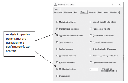
Figure 4.8 Analysis Properties Output Screen

After selecting these options, cancel out of this window and then hit the “Run Analysis” but- ton . Once the analysis is complete, you will see either an “OK” or “XX” in the “models” window. An “OK” means the model ran to completion; a “XX” means there is an error and the analysis did not finish. If an analysis is completed, you will also see the chi-square and degrees of freedom listed in the “Computational Summary” window.

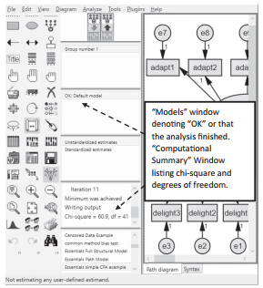
Figure 4.9  Models and Computational Summary Window

Figure 4.10 Example of Analysis Failing to Run to Completion

Let’s now take a look at the output. To get to the output results, you need to hit the “View Text”  button.This icon looks similar to the data file icon; make sure you choose the right one. Once selected, the output will come up in a separate window.You can see on the left-hand side links to different output results. The first link is “Analysis Summary”, and this just gives the time and date of analysis (not that useful). The next link is “Notes for Group”. This link will state your sample size and if the model is recursive or non-recursive. In a CFA, you should never have a non-recursive model. More information on what a non-recursive model is appears on page 310.

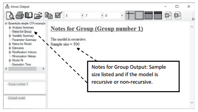
Figure 4.11 Notes for Group Output

The next tab is “Variable Summary”. An example of the output is provided in Figure 4.12. This is a breakdown of your model that lists each variable and if it is an independent or depend- ent variable.You will see that all unobserved latent variables and all error terms in the CFA analysis are listed as independents and all indicators are listed as dependent variables.

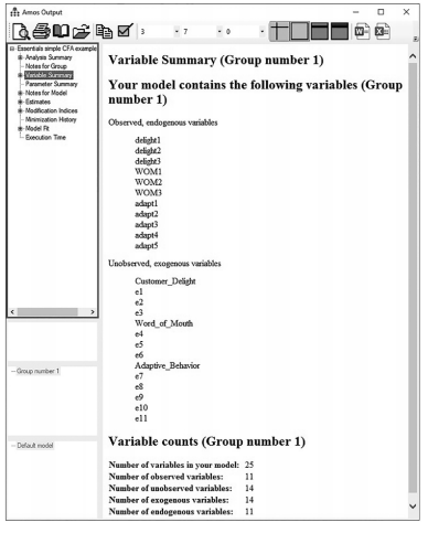
Figure 4.12 Variable Summary Output

The next link is “Parameter Summary”. This is a detailed breakdown of all the parameters in your model.

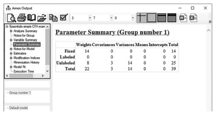
Figure 4.13 Parameter Summary Output

Next is the “Notes for Model” link; this will list your degrees of freedom in your model along with the chi-square test.The Notes for Model output will also be where AMOS presents error messages if your model does not run to completion.

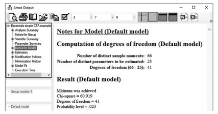
Figure 4.14 Notes for Model Output

The next tab is the “Estimates” tab.This tab is where a lot of the information you need will be located. In the Estimates tab, you will find the unstandardized and standardized regres- sion weights (for a CFA, these are referred to as factor loadings).The first regression weights presented are the unstandardized regression weights. Next, you will see the column “S.E.”, which stands for Standard Error.The next column is the critical ratio (C.R.); this is the t-value to determine significance.The next column is the p-value. If the p-value is under .001, it will just be listed as stars. Right under the unstandardized regression weights is the standardized regression weights.You will notice that it does not include C.R. or p-values.These values are the same as the unstandardized values above. Normally, in a CFA, you present standardized regression weights (factor loadings) along with the t-values for each. You need to pay close attention that you choose the corresponding t-value from the unstandardized regression output when presenting the standardized factor loadings and t-values. After the standardized weights, the “Estimates” tab will provide information on your covariances and correlations. These values can help determine if you have a possible multicollinearity issue. At the bottom of the page will be the squared multiple correlations (R2). If you remember from earlier, this is nothing more than a standardized regression weight that is squared. For a full example of the “Estimates” output, see Figure 4.15.

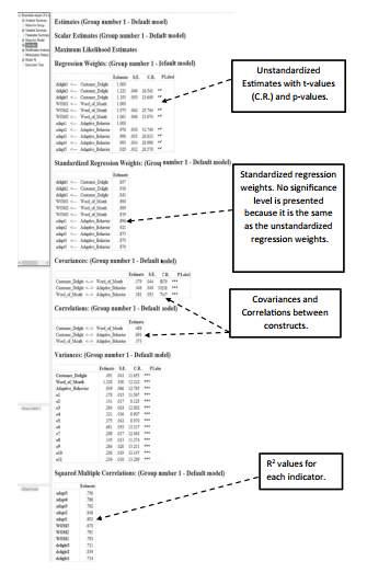
Figure 4.15 Estimates Output in AMOS

The next tab I want to discuss is the “Model Fit” tab.This tab provides you with a list of vari- ous model fit indices. On the first line, you will see NPAR, which stands for number of param- eters.The next column, CMIN, is your chi-square value, while DF is the degrees of freedom in the model and P is the p-value for a chi-square test.The last column, CMIN/DF, is the relative chi-square test or, specifically, chi-square divided by the number of degrees of freedom. In this tab, your model will be listed as the “Default” model. AMOS gives you an overabundance of fit tests, but I will highlight here the ones I think are most relevant.

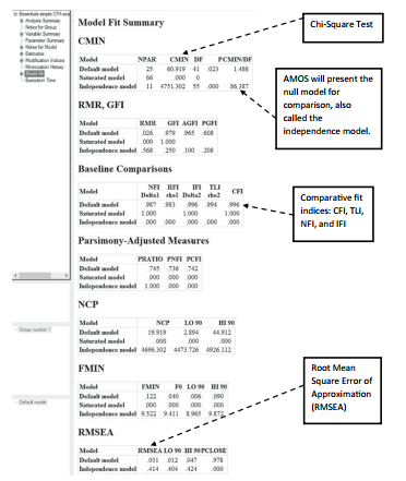
Figure 4.16 Model Fit Output

Below the Estimates tab in the output is the “Modification Indices” tab (you will see this tab only if you requested this in the Analysis Properties Window). The values listed are modifica- tions for possible covariances and also modifications if a regression weight (path) was added. With the covariances data, the M.I. value is how much the chi-square value would decrease if you added the covariance. The second column “Par Change” is how much a parameter would change if this covariance was added. See Figure 4.17.

Figure 4.17 Modification Indices Output

The last links to be discussed in the output are “Execution Time” and “Minimization His- tory”. The execution time tab tells you how long the analysis took, which is not that useful. The minimization history tab tells you how many iterations were needed for the analysis to come to completion. Neither of these links is especially pertinent when it comes to reporting results.

Overall, if we look at the results from the CFA, we can be encouraged that each unob- servable construct is being reflected in its indicators. From the “Estimates” tab, we can see that all of our indicators significantly loaded on the specified unobservable construct. All loadings were also at an acceptable level (> .70), which denotes that each indicator is explaining an acceptable amount of the variance. From the “Model Fit” output, we can see that the relative chi-square fit test is just above 1.0, which means an acceptable fit is achieved. As well, the comparative fit indices of CFI, TLI, and IFI are all above .90, further supporting the fit of the model to the data. Lastly, our RMSEA value is .03, providing additional support that the model “fits” the data. From this CFA, there is evidence that our indicators are measuring their intended concept.

Standardized Residuals

Along with modification indices,AMOS also provides a test of model misspecification through standardized residuals. The standardized residuals are the difference between the observed covariance matrix and the estimated covariance matrix for each pair of observed variables. You will specifically need to request for this information to be presented in the analysis of a SEM model. In the Analysis Properties Window, you will see a tab called “Output” and at the bottom of the window is a checkbox option for “Residual Moments”. You will need to select this box to see the Standardized Residuals in the analysis. After running the analysis, you will need to go into the output under the Estimates link and then select the Matrices option. AMOS will provide you with the unstandardized and standardized residuals, but only the standardized residuals need to be examined. Because the data is standardized, the unit of measurement is transformed to allow for easier comparison. If a residual value exceeds 2.58, then the residual of the observed and estimated covariance matrix is determined to be large (Joreskog and Sorbom 1988) and a sign of possible model misspecification. In the example output (see Figure 4.18), you can see that the biggest residual is 1.199, the difference of delight3 and adapt4.These indicators are across constructs, so no adjustment would be made in this instance. If the high residual value was within construct, then you would consider add- ing a covariance between the constructs’ error terms.

Figure 4.18 Standardized Residuals Output

Source: Thakkar, J.J. (2020). “Procedural Steps in Structural Equation Modelling”. In: Structural Equation Modelling. Studies in Systems, Decision and Control, vol 285. Springer, Singapore.