Assessing Convergent and Discriminant Validity of Your Measures in SEM Model

After initially establishing that each indicator is loading on its respective construct and the model has an acceptable fit to the data, we now need to assess the convergent and discri- minant validity of your measures. Just to recap, the basic difference between convergent and discriminant validity is that convergent validity tests whether indicators will converge to measure a single concept, whereas discriminant validity tests to see if a construct is unrelated or distinguishes from other constructs. A CFA is a good first step in determining validity, but the results of a CFA alone will not be able to confirm convergent and discrimi- nant validity.The framework outlined by Fornell and Larcker (1981) is an excellent method for assessing this type of validity and is one of the most widely used approaches with many researchers today.

To assess convergent validity, Fornell and Larcker state that you need to calculate the Aver- age Variance Extracted (AVE) for each construct. An AVE is calculated by getting the R2 value for each indicator in a construct, adding them together, and dividing by the total number of indicators. The AVE number needs to be higher than .50 to denote that your indicators have convergent validity on your construct.

With discriminant validity, you need to calculate the shared variance between constructs. To get this shared variance, a correlation analysis needs to be done between constructs (not indicators, but constructs). To perform a correlation analysis between constructs, you first need to form a composite variable for each construct. This is done by taking the scores of the indicators for each construct, summing them, and then dividing by the total number. This single composite score for each construct will be used in the correlation analysis. Once you get the correlation between constructs, you will then square those values.The resulting value should be less than the average variance extracted (AVE) for each construct. If so, you have support for discriminant validity. For simplicity, I have also seen where the square root of the AVE is compared to the original correlation of each construct. By doing it this way, you do not have to square every correlation, which could be a large number with a big model. Let’s look at an example and calculate the AVEs for our constructs used in the CFA analysis.

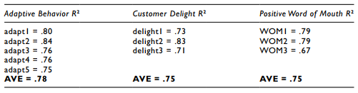
With all the AVEs for each construct having a value greater than .50, there is support that there is convergent validity for the indicators of each unobservable variable. After assessing convergent validity, let’s now investigate the discriminant validity of the constructs. The first thing we need to do is create a composite score for each construct.We will do this in the SPSS data file.

In SPSS, you need to go to the “Transform” menu at the top and then select “Compute Vari- able”. Let’s start by computing the composite variable for Adaptive Behavior. The first thing you need to do is create a new name for the composite variable. I have called the new variable “comp_adapt”, which denotes composite variable of the Adaptive Behavior construct. Next, you need to go to the “Numeric Expression” box, where you will input the formula desired. We want to initially sum all the adapt (1–5) indicators.You can select an indicator and then use the arrow key to insert that variable name in the numeric expression window. This just keeps you from having to type in all the names manually. Once you have denoted that all adapt indicators should be summed (make sure to put a parenthesis around the summation), then you need to divide by the total number of indicators. Once you hit the “OK” button at the bot- tom, SPSS will form the composite variable in the last column of your data file.You will need to repeat these steps for all the other constructs so we can perform a correlation analysis with all the composite variables that are formed.

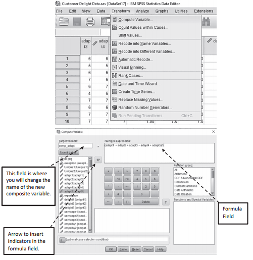
Figure 4.19  Compute Composite Variable

Here is an example of a correlation analysis with our three composite constructs.

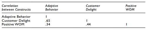To determine the shared variance between each construct, you will square the correlations and compare them to the AVE values for each construct. Let’s examine the discriminant validity of Adaptive Behavior. The shared variance between Adaptive Behavior and Customer Delight is (.65)² = .42, which is far lower than the AVE for Adaptive Behavior (.78) or Customer Delight (.75).Thus, there is evidence that these constructs discriminate from one another. Similarly, the shared variance between Adaptive Behavior and Positive Word of Mouth (.34)² = .11 is lower than the AVE values for either construct.You will need to examine every correlation and perform this comparison of shared variance to AVE to determine if you have any discriminant validity problems in your model. With our current example, all AVE values exceed the shared variance between constructs, thus supporting the discriminant validity of our constructs in the model.

Heterotrait-Monotrait Ratio of Correlations (HTMT)

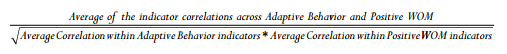
While Fornell and Larcker’s (1981) recommendation of examining shared variance to assess discriminant validity has been extremely popular in the past, recent research has started to question how sensitive this test is in capturing discriminant validity issues between constructs (Henseler et al. 2015). Subsequently, the heterotrait-monotrait ratio of correlations (HTMT) technique was offered as a better approach to determine discriminant validity between con- structs. The HTMT method examines the ratio of between-trait correlations to within-trait correlations of two constructs. Put another way, it examines the correlations of indicators across constructs to the correlations of indicators within a construct. The mathematical for- mula for HTMT is:

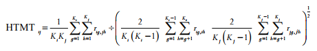
If you were like me the first time I saw that formula, you are thinking, “What in the world does all this mean?” While the formula might look a little scary, when you break it down into its parts, it is pretty simple. So, let’s take this formula and put it into layman’s terms using an example. Let’s say we wanted to determine if there was any discriminant validity problems between our constructs of Adaptive Behavior and Positive Word of Mouth. The first thing we need to assess is the value for the average heterotrait correlations. This value is the average of all the correlations across indicators of Adaptive Behavior and Positive Word of Mouth. Next, we need to determine the average monotrait correlation value.You will have an average monotrait correlation value for each of your constructs.This is the average of the correlations of indicators within a construct. So, let’s look at our formula again in a simplified form.

HTMT Formula:

Let’s look at the correlation matrix of the two construct’s indicators to help clarify the issue.

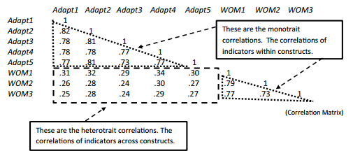
Figure 4.20 HTMT Correlations

Heterotrait Correlations:

.31 + .32 + .29 + .34 + .30 + .26 + .28 + .24 + .30 + .27 + .25 + .28 + .24 + .29 +.27 = 4.24/15

Average Heterotrait correlation = .282

Monotrait Correlations:

Adaptive Behavior = .82 + .78 + .78 + .77 + .81 + .78 + .81 + .77 + .73 + .77 = 7.82/10

Average monotrait correlation for Adaptive Behavior = .782

PositiveWord of Mouth = .79 + .77 + .73 = 2.29/3

Average monotrait correlation for Positive Word of Mouth = .763

The HTMT value across the Adaptive Behavior and Positive Word of Mouth constructs is .365. Kline (2011) states that if a HTMT value is greater than .85, then you have discriminant validity problems. Values under .85 indicate that discriminant validity is established and the two constructs are distinctively different from one another. In our example, we can conclude that discriminant validity has been established across the constructs of Adaptive Behavior and Positive Word of Mouth. If you had other constructs in your model, you would need to get an HTMT value for each pair of constructs to show discriminant validity across your model.

I would love to tell you that AMOS has an easy function to handle HTMT, but right now it does not. Hand calculating HTMT is a little tedious, and there are other options.You can get your correlation matrix and import it into an Excel spreadsheet and then highlight the cells you need to average.This is a little quicker than doing it by hand.There is also a plugin, created for AMOS by James Gaskin, that will calculate all the HTMT values in a model. That plugin can be found at http://statwiki.kolobkreations.com/index.php?title=Main_Page. There is a growing trend to use the HTMT method to assess discriminant validity because it is purported to be the best balance between high detection and low false positive rates in determining the discriminant validity of a construct (Voorhees et al. 2016).

Source: Thakkar, J.J. (2020). “Procedural Steps in Structural Equation Modelling”. In: Structural Equation Modelling. Studies in Systems, Decision and Control, vol 285. Springer, Singapore.