Computing g from Commonly Reported Results

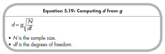
As when computing r, you can compute standardized mean differences from a wide range of commonly reported information. Although I have presented three different types of standardized mean differences (g, d, and gGlass), I describe only the computation of g in detail in the following. If you are inter­ested in using gGlass as the effect size in one’s meta-analysis, the primary studies must report means and standard deviations for both groups; if this is the case, then you can simply compute gGla_ss using Equation 5.7. If you prefer d to g (although, again, they are virtually identical with larger sample sizes), then you can use the methods described in this section to compute g and then transform g into d using the following equation with no loss of precision:

1. From Descriptive Data

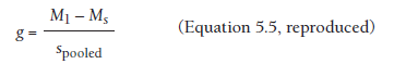
The most straightforward situation arises when the primary study reports means and standard deviations for both groups of interest. In this situation,you simply compute g directly from this information using Equation 5.5. For convenience, this equation is

 

2. From Inferential Tests

2.1. Continuous Dependent Variables

As when computing r, it is possible to compute g from the result of independent sample £-tests or 1 df F-ratios (see below for dependent sample or repeated- measures tests). For the independent sample £-test, the relevant equation is:

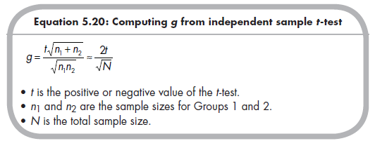
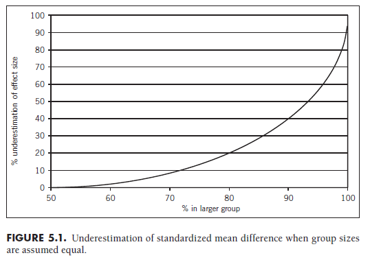
When these two group sizes are equal, this equation simplifies to the ratio on the right. In instances where the primary studies report the results of the t-test but not the sample sizes for each group (but instead only an overall sample size), this simplification can be used if the group sizes can be assumed to be approximately equal. Figure 5.1 (see similar demonstration in Rosenthal, 1991) shows the percentage underestimation in g when one incorrectly assumes that group sizes are equal. The x-axis shows the percent­age of cases in the larger group, beginning at 50% (equal group sizes) to the left and moving to larger discrepancies in group size as one moves right. It can be seen that the amount of underestimation is trivial when groups are similar in size, reaching 5% underestimation at around a 66:34 (roughly 2:1) discrepancy in group sizes. The magnitude of this underestimation increases rapidly after this point, becoming what I consider unacceptably large when group sizes reach 3:1 or 4:1 (i.e., when 75-80% of the sample is in one of the two groups). If this unequal distribution is expectable (which might be determined by considering the magnitudes of group sizes in other studies reporting sample sizes by group), then it is probably preferable to use r as an index of effect size given that it is not influenced by the magnitude of this unequal distribution.

As expected given the parallel between independent sample t-tests and two group ANOVAs, it is also possible to compute standardized mean differ­ences from F-ratios with 1 df in the numerator using the following formulas:

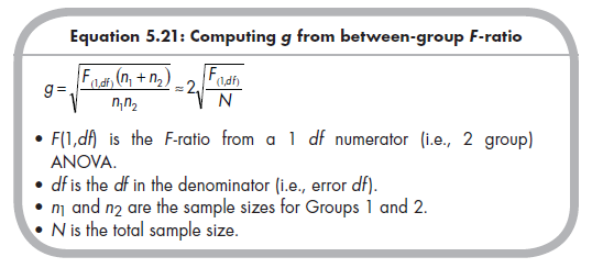
Because F-ratios are always positive, it is important that you carefully consider the direction of group differences and take the positive or negative square root of Equation 5.21, depending on whether Group 1 or 2 (respec­tively) has the higher mean.

Although computing r was equivalent whether the results were from independent (between-group) or dependent (repeated-measures) results, this is not the case when computing g. Therefore, it is critically important that you be sure whether the reported t or F values are from independent or dependent tests. If the results are from dependent, or repeated measures, tests, the following equations should be used:

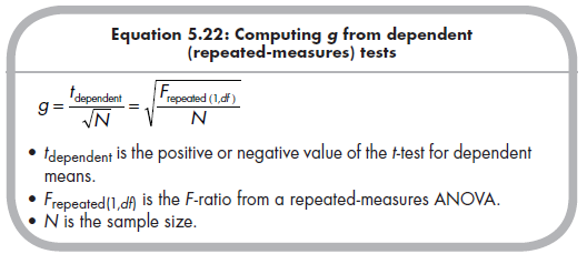
Unlike Equations 5.20 and 5.21 for the independent sample situation in which there were separate formulas for unequal and equal group sizes, the dependent (repeated-measures) situation to which Equation 5.22 applies contains only an overall N, the size of the sample over time (or other type of repeated measures). It also merits mention that the same t or F values yield a standardized mean difference that is twice as large in the independent sam­ple (between groups) than in the dependent (repeated-measures) situations, so a mistake in using the wrong formulas would have a dramatic impact on computed standardized mean effect size.

2.2. Dichotomous Dependent Variables

Primary studies might also compare two groups on the percentage or propor­tion of participants scoring affirmative on a dichotomous variable. This may come about either because the primary study authors artificially dichoto­mized the variable or because the variable truly is dichotomous. If the latter case is consistent across all studies, then you might instead choose the odds ratio as a preferred index of effect size (i.e., associations between a dichoto­mous grouping variable and dichotomous measure). However, there are also instances in which the standardized mean difference is appropriate in this situation, such as when the primary study authors artificially dichotomized the variable on which the groups are compared (in which case corrections for this artificial dichotomization might be considered; see Chapter 6), or when you wish to consider the dichotomous variable of the study in relation to a continuous variable of other studies (in which case it might be useful to consider moderation across studies using continuous versus dichotomous variables; see Chapter 10).

When two groups are compared on a dichotomous or dichotomized vari­able, you need to identify the 1 df c² and direction of effect (i.e., which group has a higher percentage or proportion). This information might be reported directly, or you may need to construct a 2 X 2 contingency table from reported results. For instance, a primary study might report that 50% of Group 1 had the dichotomous characteristic, whereas 30% of Group 2 had this characteristic; you would use this information (and sample size) to compute a contingency table and x². You then convert this x² to g using the following equation:

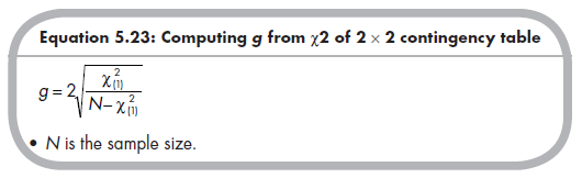
As with computing g from the F-ratio, it is critical that you take the correct positive or negative square root. The positive square root is taken if Group 1 has the higher percentage or proportion with the dichotomous characteristic, whereas the negative square root is taken if Group 2 more commonly has the characteristic.

3. From Probability Levels of Significance Tests

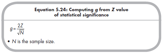
The practices of computing g from exact significance levels, ranges of signifi­cance (e.g., p < .05), and reports that a difference was not significant follow the practices of computing r described earlier. Specifically, you determine the Z for the exact probability (e.g., Z = 2.14 from p = .032), the lower-bound Z when a result is reported significant at a certain level (e.g., Z = 1.96 for p < .05), or the maximum Z when a result is reported as not significant (e.g., maximum Z = ±1.96, although the conservative choice in this option is to assume g = 0), as described in Section 5.2.4. You then use the following equa­tion to estimate the standardized mean difference from this Z: ¹³

4. From Omnibus Test Results

Although you might consider the grouping variable to most appropriately consist of two levels (i.e., two groups), there is no assurance that primary study authors have all reached the same conclusion. Instead, the groups of interest may be subdivided within primary studies, resulting in omnibus comparisons among three or more groups. For example, you might be inter­ested in comparing aggressive versus nonaggressive children, but a primary study might further subdivide aggressive children into those who are aggres­sive rarely versus frequently. Another example might be if you wish to com­pare a certain type of psychotherapy versus control, but the primary study reports results for three groups: control, treatment by graduate students, and treatment by doctoral-level practitioners. Studies might also report omnibus tests involving groups that are not of interest to a particular meta-analysis. For instance, a meta-analysis comparing psychotherapy versus control might include a study reporting outcomes for three different groups: control, psy­chotherapy, and medication. In each of these cases, it is necessary to reorga­nize the results of the study to fit the two-group comparison of interest. Next, I describe ways of doing so from reported descriptive statistics and F-ratios with df > 2.

4.1. From Descriptive Statistics

The simplest case is when studies report sample sizes, means, and standard deviations from three or more groups. Here, you can either select specific groups or else aggregate groups to derive data from the two groups of inter­est.

When you are interested in only two groups from among those reported in a study (e.g., interested in control and psychotherapy from a study report­ing control, psychotherapy, and medication), it is straightforward to use the reported means and standard deviations from those two groups to compute g (using Equation 5.5). When doing so, it is important to code the sample size, N (used to compute the standard error of the effect size for subsequent weighting), as the combined sample sizes from the two groups of interest (N = n1 + n2) rather than the total sample size from the study.

When the primary study has subdivided one or both groups of interest, you must combine data from these subgroups to compute descriptive data for the groups of interest. For example, when comparing psychotherapy versus control from a study reporting data from two psychotherapy groups (e.g.,those being treated by graduate students versus doctoral-level practitioners), you would need to combine data from these two psychotherapy groups before computing g. Combining the subgroup sample sizes is straightforward, ngroup = nsubgroup1 + nsubgroup2. The group mean is also reasonably straightforward, as it is computed as the weighted (by subgroup size) average of the subgroup means,

The combined group standard deviation is somewhat more complex to obtain in that it consists of two components: (1) variance within each of the groups you wish to combine and (2) variance between the groups you wish to combine. Therefore, to obtain a combined group standard deviation, you must compute sums of squared deviations (SSs) within and between groups. The SSwithin is computed for each group g as sg 2*(ng – 1), and then these are summed across groups. The SSbetween is computed as S [(Mg – GM)2 * ng], (where GM is the grand mean of these two groups), summed over groups. You add the two SSs (i.e., SSwithin and SSbetween) to produce the total sum of squared deviations, SStotal. The (population estimated of the) variance for this combined group is then computed as SStotal / (ncombined – 1) and the (population estimate of the) standard deviation (scombined).

Combining more than two subgroups to form a group of interest is straightforward (e.g., averaging three or more groups). It may also be neces­sary to combine subgroups to form both groups of interest (e.g., multiple treatment and multiple control groups). Once you obtain the descriptive data (sample sizes, means, and standard deviations) for the groups of interest, you use Equation 5.5 to compute g.

4.2. From df > 2 F-Ratio

As when computing r, it is also possible to compute g from omnibus ANOVAs if the primary study reports the F-ratio and means from each group. Here, you follow the general procedures of selecting or aggregating subgroups as described in the previous section. Doing this for the sample sizes and reported means is identical to the approach described in Section 5.3.4.a. The only difference in this situation is that you must infer the within-group stan­dard deviations from the results of the ANOVA, as these are not reported (if they are, then you can simply use the procedures described in the previous subsection).

Because omnibus ANOVAs typically assume equal variance across groups, this search is in fact for one standard deviation common across groups (equivalent to a pooled standard deviation). The MS_wi_thi_n of the ANOVA represents this common group variance, so the square root of this M5_wi_thi_n represents the standard deviation of groups, which are then used as described in the previous subsection (i.e., you must still combine the SSs within and between groups to be combined). If the primary study reports an ANOVA table, you can readily find this MS_wi_thi_n within the table. If the primary study does not report this MS_within, it is possible to compute this value from the reported means and F-ratio. As described earlier, you first compute the omnibus MS_{between-omnibus} = S(Mg – GM)² / G – 1 across all groups comprising the reported ANOVA (i.e., this MSp_{etween-omnibus} rep­resents the amount of variance between all groups in the omnibus com­parison), and then compute MS_within = MS_between/F. As mentioned, you then take the square root of MS_within to obtain Sp_pooled, used in computing the SS_within of the group to be combined. It is important to note that you should add the SSp_etween of just the groups to be combined in computing the SS_totaj for the combined groups, which is used to estimate the combined group standard deviation.

Source: Card Noel A. (2015), Applied Meta-Analysis for Social Science Research, The Guilford Press; Annotated edition.