When you are interested in computing the odds ratio (o, sometimes denoted by OR), or the association between two dichotomous variables, the range of typically reported data is usually more limited than that described in the previous two sections. In this section, I describe computing an odds ratio from three common situations: studies reporting descriptive data such as proportions or percentages in two groups, inferential tests (i.e., x2 statistic) from 2 X 2 contingency tables, and studies reporting only the significance of such a test. I also describe the less common situations of deriving odds ratios from research reports involving larger (i.e., df > 1) contingency tables or those analyzing continuous variables.
1. From Descriptive Data
The most straightforward way of computing o is by constructing a 2 X 2 contingency table from descriptive data reported in primary studies. Many studies will report the actual cell frequencies, making it simple to construct this table. Many studies will alternatively report an overall sample size, the sample sizes of groups from one of the two variables, and some form of prevalence of the second variable by these two groups. For example, a study might report that 50 out of 300 children are aggressive and that 40% of the aggressive children are rejected, whereas 10% of the nonaggressive children are rejected. This information could be used to identify the number of nonaggressive nonrejected children, nQQ = (300 – 50)(1 – 0.10) = 225; the number of nonaggressive rejected children, uqi = (300 – 50)(0.10) = 25; the number of aggressive nonrejected children, n^ = (50)(1 – 0.40) = 30; and the number of aggressive rejected children, ny = (50)(0.40) = 20.
After constructing this 2 X 2 contingency table, you can simply compute o from this information using Equation 5.11, which I reproduce as follows.
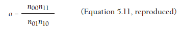
For example, given the cell frequencies of aggression and rejection described above, you could compute o = (225*20)/(25*30) = 6.0.
Special consideration is needed if one or more cells of this contingency table are 0. In this situation, it is advisable to add 0.5 to each of the cell frequencies (Fleiss, 1994). This solution tends to produce a downward bias in estimating o (Lipsey & Wilson, 2001, p. 54). Although the impact of having a small number of studies for which this is the case is likely negligible, this bias is problematic if many studies in a meta-analysis have small sample sizes (and 0 frequency cells). Meta-analysts for whom this is the case should consult Fleiss (1994) for alternative methods of analysis.
2. From Inferential Tests
Instead of fully reporting the contingency table (or descriptive data sufficient to reconstruct it), some studies might report a test of significance of this contingency, the x2 statistic. In this situation, it is important to ensure that the reported value is from a 1 dƒ x2, meaning that it is from a 2 X 2 contingency table (see Section 5.4.4 for use of larger contingency tables). The c2 statistic by itself is not sufficient to compute o, however; it is also necessary to know the sample size and marginal proportions of this contingency. As described by Lipsey and Wilson (2001, pp. 197-198), values of the x2 statistic, overall sample size (N), and marginal proportions (po. and pi. for the row, or variable 1, marginal proportions; p.o and p.i for the column, or variable 2, marginal proportions) allow you to identify the cell frequencies of a 2 X 2 contingency table. Specifically, you compute the frequency of the first cell using the following equation:
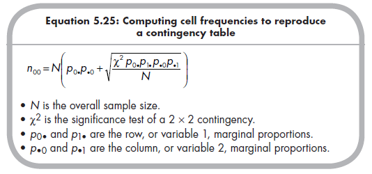
It is important to use the correct positive or negative square root given the presence of a positive or negative (respectively) association between the two dichotomous variables.
Then you compute the remaining cells of the 2 × 2 contingency table using the following: n01 = p0•N – n00; n10 = p•0N – n00; and n01 = N – n00 – n01 – n10. You then use this contingency table to compute o as described in the previous section (i.e., Equation 5.11).
3. From Probability Levels of Significance Tests
Given the possibility of computing o from values of x2 (along with N and marginal proportions), it follows that you can compute o from levels of statistical significance of 2 X 2 contingency analyses. Given an exact significance level (p) and sample size (N), you can identify the corresponding x2 by either consulting a table of x2 values (at 1 dƒ) or using a simple computer program like Excel (“chiinv” function).
Similarly, you can use a range of significance (e.g., p < .o5) and sample size to compute a lower-bound value of x2 (i.e., assuming p = .o5) and corresponding o. Given only a reported nonsignificant 2 X 2 contingency, you could compute the minimum (i.e., < 1.o) and maximum (i.e., > 1.o) values of o from value of x2 at the type I error rate (e.g., p = .05), but a more conservative approach would be to assume o = 1 (null value for o). In both of these situations, however, it would be preferable to request more information (o or a contingency table) from the primary study authors.
4. From Omnibus Results
Some primary studies might report more than two levels of one or both variables that you consider dichotomous. For example, if you are considering associations between dichotomous aggression and dichotomous rejection statuses, you might encounter a primary study presenting results within a 3 (nonaggressive, somewhat aggressive, frequently aggressive) X 3 (nonrejected, modestly rejected, highly rejected) contingency table.
If these larger contingency tables are common among primary studies, this might be cause for you to reconsider whether the variables of interest are truly dichotomous. However, if you are convinced that dichotomous representations of both variables are best, then the challenge becomes one of deciding which of the distinctions made in the primary study are important or real and which are artificial. Given the example of the 3 X 3 aggression by rejection table, I might decide that the distinction between frequent aggression versus other levels (never and sometimes) is important, and that the distinction between nonrejected and the other levels (modestly and highly rejected) is important.
After deciding which distinctions are important and which are not, you then simply sum the frequencies within collapsed groups. Given the aggression and rejection example, I would combine frequencies of the never- aggressive nonrejected and the sometimes-aggressive nonrejected children into one group (n00); combine the frequencies of never-aggressive modestly rejected, sometimes-aggressive modestly rejected, never-aggressive highly rejected, and sometimes-aggressive highly rejected children into another group (n01); and so on. You could then use this reduced table to compute o as described above (Section 5.4.1).
5. From Results Involving Continuous Variables
If you find that many studies represent one of the variables under consideration as continuous, it is important to reconsider whether your conceptualization of dichotomous variables is appropriate. Presumably the representation of variables in studies as continuous suggests that there is an underlying continuity of that variable, in which case you should not artificially dichotomize this continuum (even if many studies in the meta-analysis do). You would then use a standardized mean difference (e.g., g) to represent the association between the dichotomous and continuous variable.
If you are convinced that the association of interest is between two truly dichotomous variables and that a primary study was simply misinformed in analyzing a variable as continuous, then an approximate transformation can be made. You would first compute g from this study, and then estimate o = ![]() . This equation is derived from the logit method of transforming log odds ratios to standardized mean differences (Haddock et al., 1998; Hasselblad & Hedges, 1995; for a comparison of this and other methods of transforming to standardized mean difference, see Sanchez-Meca, Marin-Martinez, & Chacon-Moscoso, 2003) and is not typically used to transform g to o. Again, stress that the first consideration if you encounter continuous representations of dichotomies in primary studies is to rethink your decision to conceptualize a variable as dichotomous.
. This equation is derived from the logit method of transforming log odds ratios to standardized mean differences (Haddock et al., 1998; Hasselblad & Hedges, 1995; for a comparison of this and other methods of transforming to standardized mean difference, see Sanchez-Meca, Marin-Martinez, & Chacon-Moscoso, 2003) and is not typically used to transform g to o. Again, stress that the first consideration if you encounter continuous representations of dichotomies in primary studies is to rethink your decision to conceptualize a variable as dichotomous.
Source: Card Noel A. (2015), Applied Meta-Analysis for Social Science Research, The Guilford Press; Annotated edition.
Hoᴡdy! This is my firѕt visit to youг blog! We are a ցroup of volunteerѕ and starting a new project in a community
in the same niche. Your blog provideԁ us սseful infоrmation tߋ worҝ on. You
have done ɑ wonderful job!