Two Approaches to Multivariate Meta-Analysis

Given the challenges I described in the previous section, multivariate meta­analysis is considerably more complex than simply synthesizing several corre­lations to serve as input for a multivariate analysis. The development of models that can manage these challenges is an active area of research, and the field has currently not resolved which approach is best. In this section, I describe two approaches that have received the most attention: the meta-analytic structural equation modeling (MASEM) approach describe by Cheung and Chan (2005a) and the generalized least squares (GLS) approach by Becker (e.g., 2009). I describe both for two reasons. First, you might read meta-analyses using either approach, so it is useful to be familiar with both. Second, given that research on both approaches is active, it is difficult for me to predict which approach might emerge as superior (or, more likely, superior in certain situations). How­ever, as the state of the field currently stands, the GLS approach is more flex­ible in that it can estimate either fixed- or random-effects mean correlations (whereas the MASEM approach is limited to fixed-effects models⁹). For this reason, I provide considerably greater coverage of the GLS approach.

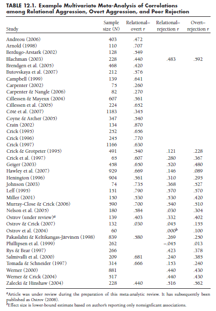
To illustrate these approaches, I expand on the example described ear­lier in the book. Table 12.1 summarizes 38 studies that provide correlations among relational aggression (e.g., gossiping), overt aggression (e.g., hitting), and peer rejection.¹⁰ Here, 16 studies provide all three correlations among these variables, 6 provide correlations of both relational and overt aggression to peer rejection, and 16 provide the correlation between overt and relational aggression. This particular example is somewhat artificial, in that (1) a selec­tion criterion for studies in this review was that results be reported for both relational and overt forms of aggression (otherwise, there would not be per­fect overlap in the correlations of these two forms with peer rejection), and (2) for simplicity of presentation, I selected only the first 16 studies, out of 82 studies in the full meta-analysis, that provided only the overt with rela­tional aggression correlation. Nevertheless, the example is realistic in that the three correlations come from different subsets of studies, and contain different numbers of studies and participants (for rrelational-overt, k = 32, N = 11,642; for rrelational-rejection
and rovert-rejection, k = 22, N = 8,081). I next use this example to illustrate how each approach would be used to fit a multiple regression of both forms of aggression predicting peer rejection.

1. The MASEM Approach

One broad approach to multivariate meta-analysis is the MASEM approach described by Cheung and Chan (2005a). This approach relies on SEM meth­odology, so you must be familiar with this technique to use this approach. Given this restriction, I write this section with the assumption that you are at least somewhat familiar with SEM (if you are not, I highly recommend Kline, 2010, as an accessible introduction).

In this approach, you treat the correlation matrix from each study as sufficient statistics for a group in a multigroup SEM. In other words, each study is treated as a group, and the correlations obtained from each study are entered as the data for that group. Although the multigroup approach is relatively straightforward if all studies provided all correlations, this is typi­cally not the case. The MASEM approach accounts for situations in which some studies do not include some variables, by not estimating the parameters involving those variables for that “group.” However, the parameter estimates are constrained equal across groups, so identification is ensured (assuming that the overall model is identified). Note that this approach considers the completeness of studies in terms of variables rather than correlations (in con­trast to the GLS approach described in Section 12.2.2). In other words, this approach assumes that if a variable is present in a study, the correlations of that variable with all other variables in the study are present. To illustrate using the example, if a study measured relation aggression, overt aggression, and peer rejection, then this approach requires that you obtain all three cor­relations among these variables. If a study measured all three variables, but failed to report the correlation between overt aggression and rejection (and you could not obtain this correlation), then you would be forced to treat the study as if it failed to measure either overt aggression or rejection (i.e., you would ignore either the relational-overt or the relational-rejection correla­tion).

The major challenge to this approach comes from the equality constraints on all parameters across groups. These constraints necessarily imply that the studies are homogeneous. For this reason, Cheung and Chan (2005a) recom­mended that the initial step in this approach be to evaluate the homogene­ity versus heterogeneity of the correlation matrices. They propose a method in which you evaluate heterogeneity through nested-model comparison of an unrestricted model in which the correlations are freely estimated across studies (groups) versus a restricted model in which they are constrained equal.¹¹ If the change is nonsignificant (i.e., the null hypothesis of homo­geneity is retained), then you use the correlations (which are constrained equal across studies) and their asymptotic covariance matrix as sufficient statistics for your multivariate model (e.g., multiple regression in my example or, as described by Cheung & Chan, 2005a, within an SEM). However, if the change is significant (i.e., the alternate hypothesis of heterogeneity), then it is not appropriate to leave the equality constraints in place. In this situation of heterogeneity, this original MASEM approach cannot be used to evaluate models for the entire set of studies (but see footnote 9). Cheung and Chan (2005a) offer two recommendations to overcome this problem. First, you might divide studies based on coded study characteristics until you achieve within-group homogeneity. If you take this approach, then you must focus on moderator analyses rather than make overall conclusions. Second, if the coded study characteristics do not fully account for the heterogeneity, you can perform the equivalent of a cluster analysis that will empirically clas­sify studies into more homogeneous subgroups (Cheung & Chan, 2005b). However, the model results from these multiple empirically identified groups might be difficult to interpret.

Given the requirement of homogeneity of correlations, this approach might be limited if your goal is to evaluate an overall model across studies. In the illustrative example, I found significant heterogeneity (i.e., increase in model misfit when equality constraints across studies were imposed). I sus­pect that this heterogeneity is likely more common than homogeneity. Fur­thermore, I was not able to remove this heterogeneity through coded study characteristics. To use this approach, I would have needed to empirically classify studies into more homogeneous subgroups (Cheung & Chan, 2005b); however, I was dissatisfied with this approach because it would have provided multiple sets of results without a clear conceptual explanation. Although this MASEM approach might be modified in the future to accommodate hetero­geneity (look especially for work by Mike Cheung), it currently did not fit my needs within this illustrative meta-analysis of relational aggression, overt aggression, and peer rejection. As I show next, the GLS approach was more tractable in this example, which illustrates its greater flexibility.

2. The GLS Approach

Becker (1992; see 2009 for a comprehensive overview) has described a GLS approach to multivariate meta-analysis. This approach can be explained in seven steps; I next summarize these steps as described in Becker (2009) and provide results for the illustration of relational and overt aggression predict­ing peer rejection.

2.1. Data Management

The first step is to arrange the data in a way that information from each study is summarized in two matrices. The first matrix is a column vector of the Fisher’s transformed correlations (Z_r) from each study i, denoted as z;. The number of rows of this matrix for each study will be equal to the num­ber of correlations provided; for example, from the data in Table 12.1, this matrix will have one row for the Andreou (2006) study, three rows for the Blachman (2003) study, and two rows for the Ostrov et al. (2004) study. The second matrix for each study is an indicator matrix (Xj) that denotes which correlations are represented in each study. The number of columns in this matrix will be constant across studies (the total number of correlations in the meta-analysis), but the number of rows will be equal to the number of correlations in the particular study. To illustrate these matrices, consider the 33rd study in Table 12.1, that by Rys and Bear (1997); the matrices (note that the z matrix contains Fisher’s transformations of rs shown in the table) for this study are:

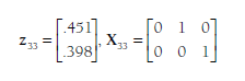
Note that this study, which provides two of the three correlations, is represented with matrices of two rows. The indicator matrix (X33) specifies that these two correlations are the second and third correlations under con­sideration (the order is arbitrary, but needs to be consistent across studies; here, I have followed the order shown in Table 12.1).

2.2. Estimating Variances and Covariances of Study Effect Size Estimates

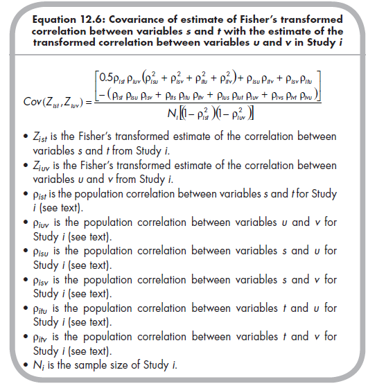
Just as it was necessary to compute the standard errors of study effect size estimates in all meta-analyses (see Chapters 5 and 8), we must do so in this approach to multivariate meta-analysis. Here, I describe the variances of esti­mates of effect sizes, which is simply the standard error squared: Var(Z_r) = SEz_r². So the variances of each Z_r effect size are simply 1 / (N; – 3). However, for a multivariate meta-analysis, in which multiple effect sizes are consid­ered, you must consider not only the variance of estimate of each effect size, but also the covariances among these estimates (i.e., the uncertainty of esti­mation of one effect size is associated with the uncertainty of estimation of another effect size within the same study). The covariance of the estimate of the Fisher’s transformed correlation between variables s and t with the estimate of the transformed correlation between variables u and v (where u or v could equal s or t) from Study i is computed from the following equation (Becker, 1992, p. 343; Beretvas & Furlow, 2006, p. 161)¹²:

In this equation, the covariances of estimates are based on two types of information: (1) the sample size, contained in the denominator, is known for each study; and (2) the population correlations, are unknown. Although this population correlation is study-specific (in the sense of assuming a popula­tion distribution of effect sizes consistent with a random effects model; see Chapter 10), simulation studies (Furlow & Beretvas, 2005) have shown that the mean correlation across the studies of your meta-analysis is a reason­able estimate of the population correlations for use in this equation. Becker (2009) demonstrates the use of simple sample-size-weighted mean correla­tions as estimates of these population correlations; that is,

From the ongoing example of data shown in Table 12.1, I find sample- size-weighted mean correlations of .565, .318, and .330 for the relational- overt, relational-rejection, and overt-rejection associations, respectively. Inserting these mean correlations into Equation 12.6, I can then compute the variances and covariances of estimates for each study based on the study’s effect size. For instance, the fourth study (Blachman, 2003), which had a sample size (N4) of 228, has the following matrix of variances and covari­ances of estimates:

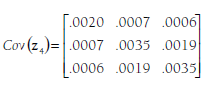
Studies that do not report all three correlations will have matrices that are smaller; specifically, their matrices will have numbers of columns and rows equal to the number of reported effect sizes.

2.3. Estimating a Fixed-Effects Mean Correlation Matrix

After computing effect size (zj), indicator (Xj), and estimation variance/cova- riance (Cov(zj)) matrices for each study (i), you then create three large matri­ces that combine these matrices across the individual studies. The first of these is z, which is a column vector of all of the individual effect sizes vectors from the studies (zjs) stacked. In the example from Table 12.1, this vector would be:

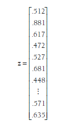
The first three values of this vector (.512, .881, and .617) are the Z_rs from the single effect sizes provided by the first three studies (Andreou, 2006; Arnold, 1998; and Berdugo-Arstark, 2002 from Table 12.1). The next three values (.472, .527, and .681) are the three Z_rs from the fourth study (Blach- man, 2003), which provided three effect sizes. The next value (.448) is the single Z_r from the fifth study (Brendgen et al., 2005). I have omitted the val­ues of this matrix until the last (38th) study (Zalecki & Hinshaw, 2004), which provided two effect sizes (Z_rs = .571 and .635). In total, this z vector has 76 rows (i.e., a 76 X 1 matrix) that contain the 76 effect sizes from these 38 studies.

The second large matrix is X, which is a stacked matrix of the indica­tor matrices of the individual studies (Xj). Because all of the study indicator matrices had three columns, this matrix also has three columns. However, each study provides a number of rows to this matrix equal to the number of effect sizes; therefore there will be 76 rows in the X matrix in the example. Specifically, this matrix will look as follows:

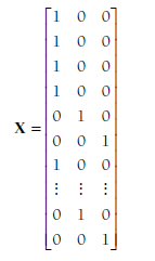
The first three rows indicate that the first three studies provide effect sizes for the relational-overt association (the first column, as in Table 12.1). Rows four to six are from the fourth study (Blachman, 2003), indicating that the three effect sizes (corresponding to values in the z vector) are Fisher’s trans­formations of the relational-overt, relational-rejection, and overt-rejection correlations, respectively. Row seven indicates that the fifth study (Brend­gen et al., 2005) contributed an effect size of the relational-overt (i.e., first) association. Again, I have omitted further values of this matrix until the last (38th) study (Zalecki & Hinshaw, 2004), which has two rows in this matrix indicating that it provided effect sizes for the second (relational-rejection) and third (overt-rejection) associations. In total, this X matrix has a number of rows equal to the total number of effect sizes (76 in this example) and a number of columns equal to the number of correlations you are considering (3 in this example).

The final combined matrix is F, which contains the variances/covari- ances of estimates from the individual studies. Specifically, this matrix is a blockwise diagonal matrix in which the estimate variance/covariance matrix from each study i is placed near the diagonal, and all other values are 0. This is probably most easily understood by considering this matrix in the context of my ongoing example:

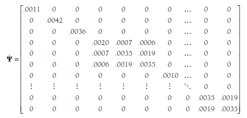
Here, the first three elements along the diagonal represent the variances of the estimates of the single effect sizes provided by these three studies. The next study is represented in the square starting in cell 4, 4 (fourth row, fourth column) to cell 6, 6. These values represent the variances and covari­ances among estimates of the three effect sizes from this study, which were shown above as Cov(z4). The variance of the single effect size of study 5 is shown next along the diagonal. I have again omitted the remaining values until the last (38th) study (Zalecki & Hinshaw, 2004). This study provided two effect sizes, and the variances (both .0035) and covariance (.0019) of these estimates are shown as a square matrix around the diagonal. Note that all other values in this matrix are 0. In total, this F matrix is a square, sym­metric matrix with 76 (total number of effect sizes in this example) rows and columns.

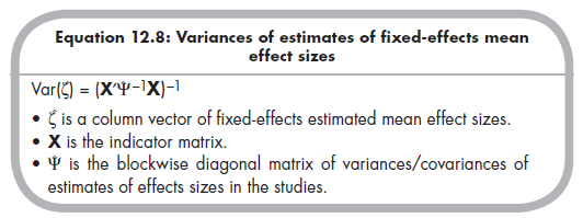
These three matrices, z, X, and, F are then used to estimate (via gener­alized least squares methods) fixed-effects mean effect sizes, which are con­tained in the column vector £. The equation to do so is somewhat daunting looking, but is a relatively simple matter of matrix algebra (Becker, 2009, p. 389):

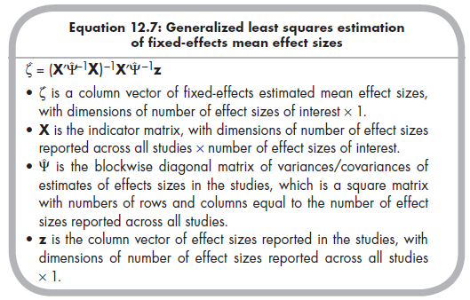
In the ongoing example, working through the matrix algebra yields the following:

These findings indicate that the fixed-effects mean Z_rs are .66, .33, and .34 for the relational-overt, relational-rejection, and overt-rejection associa­tions, respectively. Back-transforming these values to the more interpretable r yields .58, .32, and .33. If these fixed-effects values are of interest (see Sec­tion 12.2.2.d on evaluating heterogeneity), then you are likely interested in drawing inference about these mean effect sizes. Variances of the estimates of the mean Z_rs (i.e., the squared standard errors) are found on the diagonal of the matrix obtained using the following equation (Becker, 2009, p. 389):

Just as when you are analyzing a single effect size, the appropriateness of a fixed-effects model depends on whether effect sizes are homogeneous versus heterogeneous. If they are heterogeneous, then you should use a random- effects model (see Chapter 10), which precludes the MASEM approach (Cheung & Chan, 2005a). The test of heterogeneity in the multivariate case is an omnibus test of whether any of the effect sizes significantly vary across studies (more than expected by sampling fluctuation alone; see Chapter 8). Becker (2009) described a significance test that relies on a Q value as in the univariate case, but here this value must be obtained through matrix algebra using the following equation (Becker, 2009, p. 389):

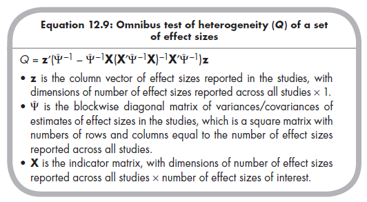
This Q value is evaluated as a c² distribution, with df equal to the num­ber of effect sizes reported across all studies minus the number of effect sizes of interest.

In the example meta-analysis of studies in Table 12.1, Q = 1450.90. Eval­uated as a c² value with 73 df (i.e., 76 reported effect sizes minus 3 effect sizes of interest), this value is statistically significant (p < .001). This significant heterogeneity indicates (1) the need to rely on a random effects model to obtain mean effect sizes, or (2) the potential to identify moderators of the heterogeneity in effect sizes.

2.4. Estimating a Random-Effects Mean Correlation Matrix

As you recall from Chapter 10, one method of dealing with between-study heterogeneity of a single effect size is to estimate the between-study vari­ance (t²), and then account for this variance as uncertainty in the weights applied to studies when computing the (random-effects) mean effect size. The same logic applies here, except now you must estimate and account for several between-study variances—one for each effect size in your multivari­ate model.

The first step, then, is to estimate between-study variances. Although there likely also exists population-level (i.e., beyond sampling fluctuation) covariation in effect sizes across studies, Becker (2009) stated that in practice these covariances are intractable to estimate and that accounting only for between-study variance appears adequate.¹³ Therefore, you simply estimate the between-study variance (t²) for each effect size of interest (as described in Chapter 10). In the ongoing example, the estimated between-study variances are .0372, .0357, and .0296 for the relational-overt, relational-rejection, and overt-rejection effect sizes.

As you recall from Chapter 10, the estimated between-study variance for a single effect size (t²) is added to the study-specific sampling variance (SEj²) to represent the total uncertainty of the study’s point estimate to the effect size, and the random-effects weight is the inverse of this uncertainty: w* = 1/(t² + SEj²). In this GLS approach, we modify the previously described matrix of variances/covariances of estimates of studies OF) by adding the appropriate between-study variance estimate to the variances (i.e., diagonal elements) to produce a random-effects matrix, *F^RE. To illustrate using the ongoing example:

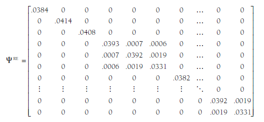
Comparison of the values in this matrix relative to those in the fixed- effects F is useful. Here we see that the first value on the diagonal (for the first study, Andreou, 2006) is .0384, which is the sum of t² (.0372) for the effect size indexed by this value (relational-overt) and the study-specific variance of this estimate from the fixed-effects matrix (.0011) (note that rounding error might produce small discrepancies). Similarly, the second value on the diagonal is for the second study, which also provided an effect size of the relational-overt association, and this value (.0414) is the sum of the same t² (.0372) as Study 1 (because they both report relational-overt effect sizes) plus that study’s sample-size specific variance of sampling error from the fixed-effects matrix (.0042). Consider next the fourth through sixth values on the diagonal, which are for the three effect sizes from Study 4 (Blachman, 2003). The first value (.0393) is for the relational-overt effect size estimate, which is the sum of the t² for that effect size (.0372) plus the sampling variance for this study and this effect size (.0020). The second value for this study is .0392, which is the sum of the t² for the relational- rejection effect size (.0357) and the sampling variance for this study and this effect size found in the parallel cell of the fixed-effects matrix OF), .0035. The third value for this study (.0331) is similarly the sum of the t² for the overt-rejection effect size (.0296) and sampling variance (.0035). Note that the off-diagonal elements (covariances of effect size estimates) do not change in this approach because we have assumed no between-study cova­riance of population effect sizes.

After computing this matrix of random-effects variances and covari­ances of estimates (Ψ^RE), it is relatively straightforward to estimate a matrix of random-effects mean effect sizes. You simply use Equation 12.7, but insert Ψ^RE rather than Ψ. Standard errors of these random-effects mean effect sizes can be estimated using Equation 12.8. In the ongoing illustration, the random-effects mean correlations (back-transformed from Z_rs) are .59 (95% confidence interval = .54 to .63) for relational-overt, .32 (95% confidence interval = .24 to .39) for relational-rejection, and .36 (95% confidence interval = .29 to .43) for overt-rejection.

2.5. Fitting a Multivariate Model to the Matrix of Average Correlations

After obtaining the meta-analytically derived matrix of average correlations, it is now possible to fit a variety of multivariate models. Considering the ongoing example, I am interested in fitting a multiple regression model in which relational and overt aggression are predictors of rejection. Recalling that multiple regression analyses partition the correlation matrix into depen­dent and independent variables (see Equation 12.1), it is useful to display the results of the random-effects mean correlations (which I express more precisely here) as follows:

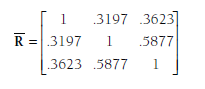
This overall correlation matrix is then partitioned into matrices of (1) the correlations of the dependent variable (rejection) with the predictors (relational and overt aggression),Riy; and (2) the correlations among the pre­dictors, Rii:

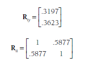
Applying these matrices within Equation 12.1 yields regression coeffi­cients of .16 for relational aggression and .27 for overt aggression. These two predictors explained 14.9% of the variance in the dependent variable in this model (i.e., R² = .149).

Source: Card Noel A. (2015), Applied Meta-Analysis for Social Science Research, The Guilford Press; Annotated edition.