Correlations Between Constructs in SEM Model

While directionality is calculated with a covariance analysis, the strength of the relationships is determined through a correlation analysis. A correlation between two concepts is essentially derived from the covariance. With a covariance analysis, the calculated values do not have a definable range or limit. If you have two variables that are measured on completely different scales, such as our previous example with number of ads and total sales, then the covariance can be a very large (or small) number that is difficult to interpret. A correlation will take that covariance value and standardize it by converting the score on to a −1 to a +1 scale. By limit- ing the values to a −1 to a +1 scale, you can now compare the strength of relationships that have all been put on a similar scale. If a correlation has a −1 value, this means that the two vari- ables have a strong inverse (negative) relationship, whereas when one variable increases, the other variable decreases. A correlation of +1 means two variables have a positive relationship where both variables are moving in the same direction at roughly the same rate. If you have a correlation value of zero, this means that the two variables are independent of one another and have no pattern of movement across the variables.

Following our same example from the covariance discussion, let’s now determine the cor- relation of number of ads placed in a week and a business’s total sales. The formula for calcu- lating a correlation coefficient is a little more straightforward than the covariance formula.To calculate a correlation, you use the following formula:

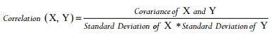
You will also see this formula represented as:

The lowercase “r” represents the correlation coefficient and the uppercase “S” represents the standard deviation of the variable. Using our previous example, if we assume the standard deviation for X (# of Ads) is 3.11 and the standard deviation for Y (total sales) is 1,844.81, then we can calculate the correlation between the two variables.

The correlation between number of ads and totals sales is .97, which shows a strong positive relationship between the two variables. Again, you will probably never hand calculate these values because we have software programs that can do the work for you in seconds. Saying that, understanding how the values are calculated can help in understanding how a SEM analy- sis is accomplished.

With SEM, you are initially going to get an “observed” sample covariance from the raw data, where you are getting a covariance across all possible combinations of variables. This observed covariance matrix will then be compared to an “estimated” covariance matrix based on your denoted model. The estimated model does not look at all possible variable combinations but solely focuses on combinations that you denote as having a relationship. For example, let’s look at a simple four variable model. In this model, the variables of Trust and Satisfaction are proposed to positively influence a consumer’s attitude toward a store. This attitude evaluation is then proposed to positively influence a consumer’s intention to shop at that store. Notice that we are proposing only three relationships across the vari- ables. See Figure 1.2.

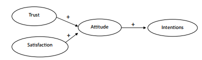
Figure 1.2 Simple Structural Model

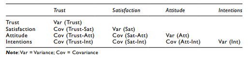
To calculate the observed covariance matrix, you would assess the variance for each vari- able and then determine the covariance for each possible variable combination. Here is an example of how the observed covariance matrix would be calculated with our four variable model.

After you have conceptualized your model, you are now going to “estimate” those specific relationships in your model to determine how well your estimated covariance matrix com- pares to the observed covariance matrix. The estimation of proposed relationships is done through a series of bivariate correlations, and the estimates will determine the strength of each relationship. These estimates are interpreted just like regression coefficients. Unlike other techniques, SEM does not treat each calculation separately. With SEM, all relationships are calculated simultaneously, thus providing a more accurate picture of the relationships denoted.

You will also see the term “model fit” used in SEM to determine how well your “esti- mated” covariance matrix (based on the denoted model) compares or fits the observed covari- ance matrix. If the estimated covariance matrix is within a sampling variation of the observed covariance matrix, then it is generally thought to be a good model that “fits the data”.

Source: Thakkar, J.J. (2020). “Procedural Steps in Structural Equation Modelling”. In: Structural Equation Modelling. Studies in Systems, Decision and Control, vol 285. Springer, Singapore.