Basics of SEM Input: The Covariance Matrix

For the purposes of this book, I will strictly use a covariance-based approach to structural equation modeling.This method is the most robust for theory testing and assessing the “struc- ture” of a specified model along with its relationships. Before we move forward, a discussion is warranted on concepts such as variance, covariance, and correlation so we are all clear on the fundamental foundation that SEM operates in the analysis.

Variance of a construct—The term variance describes how spread out the values (responses/observations) are in a concept you are measuring. You can calculate this by find- ing the mean of all your observations and then taking the distance from the mean to a record (response/observation) and squaring that value.You then take the average of all squared differ- ences from the mean to get the variance.This is usually a large number and has little interpre- tation; but if you take the square root of this number, you get the standard deviation from the mean, and this is useful. The standard deviation is typically what is used to discuss the amount of dispersion or variation in trying to measure a concept.

Covariance between constructs—Covariance is the measure of how much two vari- ables change together. If greater values of one variable correspond to greater values in another variable, you have a positive covariance. If greater values in one variable correspond to lower values in another variable, then you have a negative covariance value. The main function of a covariance analysis is to determine directionality of two variables. If the covariance is positive, then the two variables will move in the same direction. If the covariance is negative, the two variables will move in opposite directions. One of the primary assumptions in SEM is that the relationship between constructs follows a linear pattern. Put another way, if you ran a scat- ter plot of the values of two variables, the data would be in a line pattern that was increasing upward or decreasing downward. The function of a covariance analysis is simply to assess if the relationship between two variables is positive, thus having an increasing relationship, or negative and a decreasing relationship. While it is extremely unlikely that you will ever have to hand calculate a covariance value, it does provide us with a better understanding of the concept to see how the value is derived.

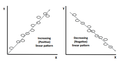
Figure 1.1 Linear Patterns

The covariance formula is: For a population:

For a sample of the population:

(The most frequently used)

I know this might look like an intimidating formula initially, but it is really not once you break down what all the symbols mean. In this formula, we are looking at the covariance value across two variables. Let’s call one of the variables “X” and the other variable “Y”. In our formula,

Xi = represents the values of the X variable

Yj = represents the values of theY variable

X¯ = represents the mean (average) of the X variable

Y¯ =  represents the mean (average) of theY variable

n = represents the total number of our sample

∑ = represents the symbol for summation

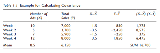
Let’s look at a quick example to clarify things. In this example, let’s say I wanted to test if the number of advertisements over a month increased a business’s sales. Each week I would need to get the number of advertisements the business placed, and the total sales at the end of the week. I would do this for four weeks.Thus, I would have four data points for this analysis. See the example in Table 1.1.

The X–X¯ value for week 1 is the number of ads (10) minus the mean (8.5) over the week = 1.50.You would need to get this value for each week. The Y–Y¯ for week 1 is 7,000 minus the mean 6,150 = 850. Again, you would need to get the value for each week.The next step is to multiply the X–X¯ value by the Y–Y¯ value. If you sum up all these products, you get the numerator for our equation (16,700). The denominator of our equation is the total num- ber of samples subtracted by the value of 1. Thus,

Our covariance value is 5,566.67. This positive value lets us know that the relationship between the two variables is positive and increasing. Outside of that, the value of 5,566.67 does not give us any more information other than directionality.To determine the strength of the relationship, we will need to assess the correlation between the constructs.

Source: Thakkar, J.J. (2020). “Procedural Steps in Structural Equation Modelling”. In: Structural Equation Modelling. Studies in Systems, Decision and Control, vol 285. Springer, Singapore.