Estimation (From Sample Mean to Population Mean) of Experimental Data

As pointed out in Chapter 18, the mean is the most significant statistic of a given set. The mean of the sample set A—56.4, 57.2, 55.9, 56.2, 55.6, 57.1, and 56.6—is 56.43. This is called the sample mean, X, and when it is used as an estimator of the popula­tion mean, fl, it is referred to as the point estimate, meaning that it is not a range of fl values. The drawback to point estimation is that it does not, by itself, indicate how much confidence we can place in this number. Suppose 56.43 came out to be the mean of a set of fifty elements, instead of a set of only seven elements as above; intuitively, we would accept it with more confidence. The higher the number of elements in the sample, the higher the con­fidence, meaning the better the estimate.

We also want to look at the part played by another statistic, namely, the standard deviation, in deciding the confidence level that a sample mean commands in the analysis of results. Instead of the sample set A seen above, say we had a sample set B consist­ing of (as before) seven elements: 61.4, 60.2, 50.9, 61.3, 51.0, 57.6, and 56.2. The mean of this set is also 56.43, the same as before, but we can readily notice the difference: whereas in set A, the individual values were close to each other, in set B there is a wide variation. Between the two samples, intuitively, we place more confidence in A than in B. As is now familiar, the statistic that measures this variation is the variance, or standard deviation, which is simply the square root of the variance. In summary, we may say that, in terms of confidence, the lower the standard devi­ation of the sample, the better the estimation.

Thus, any sample, however large, cannot provide a sample mean that can be accepted with absolute confidence as equivalent to the population mean. Some error, known as the sampling error, and given by

is always likely to occur. To avoid this drawback, another method of estimating the mean, fl, is often used; it is known as interval estimation.

1. Interval Estimation

In the ideal situation, where the sample statistic is equal to the population parameter (as in the particular case we discussed for the two means), the sample statistic is said to be an unbiased esti­mator of the corresponding population parameter. But in reality, this is never likely to happen. A sample statistic, for instance the mean, is something that we can access and evaluate. By making use of it, suppose we establish an interval within which we can be confident to a specified degree that the population mean will be located; this is the process of interval estimation. The degree of confidence is expressed in terms of probability. The interval is known as the confidence interval; the upper and lower limits are known as confidence limits.

In demonstrating the methods of estimating the confidence interval for the population mean, fl, we want to distinguish three cases:

1. A large random sample (more than thirty ele­ments) is possible, and the standard deviation, O, of the population is known.
2. The sample size is more than thirty, and O is unknown.
3. The sample size is small (less than thirty ele­ments), and O is unknown.

In all three cases, we assume arbitrarily for the present demon­stration that the degree of confidence required for m is 95 percent (or 0.95).

Case 1: Sample Size Is More Than Thirty; O Is Known

From the sample, the sample mean, X, can be readily calculated. By the definition of interval estimation, X is expected to be located between the lower and the upper limits of the population mean, fl. The statistical instruments we invoke to develop the relations are (1) the Central Limit Theorem, and (2) the standard normal distribution (see Chapter 17).

According to the Central Limit Theorem, if the sample size is reasonably large (N > 30), the distribution (of many values) of ^ approximates to normal distribution with mean fl and standard deviation

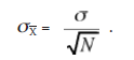
In the graphical relation of this distribution, the distance on the abscissa between fl and a particular value of X gives, in effect, the difference between the population mean, fl, and the sample mean, X. Now, adapting the notation of the standard normal dis­tribution, this difference can be represented as

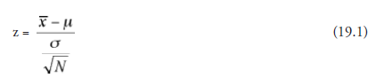
in which N is the number of elements in the sample (or simply the sample size).

It is known that the area under the curve of standard normal distribution is the numerical measure of probability, P whose maximum value is 1.0, and further that 95 percent of the area under the curve lies between the z values of -1.96 and +1.96. These facts can be formulated as

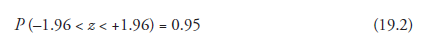
And, the verbal interpretation of this is that there is a 0.95 probability that the random variable, z, lies between -1.96 and +1.96, or (in other words) that the confidence interval for the parameter ! is 95 percent.

Combining (19.1) and (19.2), we get

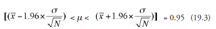
The verbal interpretation of this is that there is a 0.95 proba­bility that ! lies between

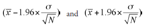
In other words, the confidence interval for the parameter fl, between the above two limits, is 95 percent.

Example with hypothetical numbers:

Sample size, N = 64

Sample mean, X (calculated) = 26.4

Standard deviation, O (known) = 4

Degree of confidence, selected = 0.95 (95 percent)

Using (19.3)

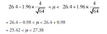
By this, we understand that the true value of fl, the popula­tion mean, lies somewhere between 25.42 and 27.38 and that we can be 95 percent confident in accepting this.

Application:

The situation in which the standard deviation of the population is known but its mean is unknown, hence, needs to be estimated, is not very likely to be encountered with the data obtained from laboratory experiments in science or engineering. On the other hand, relative to data obtained from surveys in a national census, public statistics, psychology, medicine, education, and so forth, the situation as mentioned above is likely to occur. For instance, the standard deviation in the height of adult males in the United States established last year or the year before is likely to hold good this year as well. Also, in surveys of this kind, the sample size is usually large, and the assumption made to this effect is justified.

2. Variations in Confidence Interval

In the foregoing discussion and example, we arbitrarily chose the level of confidence to be 95 percent. It is possible, for instance, to choose it to be 99 percent (or any other number). Supposing it is 99 percent, the change required is as follows: Going to the table of standard normal distribution, we select the z value such that the area under one half of the curve (because the curve is sym­metrical) is 0.99 * 2 = 0.495. That is found to be 2.575. Using the same data as in the above example, the new relation is

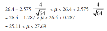
We notice that if we require a higher degree of confidence (99 percent instead of 95 percent), we end up with a wider confidence interval. It is desirable to have a combination of a higher degree of confidence and a narrower confidence interval. To look for the variables that influence these two somewhat conflicting outcomes, we go to (19.3) and note the following: Retaining a higher degree of confidence, to narrow the confidence interval, we need to increase the factor to the left of μ and decrease the factor to the right of μ. X being common to both sides, and σ being known and fixed, the only changeable factor is √N , or N, the sample size. To the extent that N, the number of elements in the sample, is higher, the lower limit of the confidence range (on left) increases and the upper limit (on the right) decreases, both together rendering the confidence range narrower. This confirms what we mentioned earlier—that larger samples should give us more confidence in estimating the population parameters. Incidentally, also note that if σ, the standard deviation, were given to be lower (say two instead of four in the example we considered), the effect would have been similar to having higher N, namely, rendering the confidence interval narrower.

Case 2: Sample Size Is More Than Thirty; s_x Is Unknown

Standard deviation of the sample, sx, is computed and substituted in place of σ in (19.3):

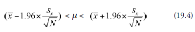
The result of the procedure is the same as in Case 1.

Application:

This is more realistic than Case 1 and suitable to laboratory experiments.

Case 3: Sample Size Is Small (Less Than Thirty); S_x Is Unknown

Like in Case 2, S_x is computed and substituted in place of O in (19.3). But that is not all; other changes follow. In place of the inequality part in (19.3) (contained within parenthesis), we need to use a modified format, namely,

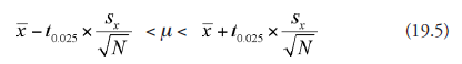
wherein we find t0.025 replacing 1.96, because instead of the standard normal distribution curve, we are required to use here what is known as the t-distribution curve. The area under this curve between the limits –t0.025 and +t0.025, like before, is 0.95, thus is the measure of confidence level required. The “0.025” in “t0.025” is derived as (1 – 0.95) ÷ 2 = 0.025: this is because the t-distribution curve, like the standard normal distribution curve, is symmetrical and “two tailed.”. At this point, we go to the t-distribution table (Table 18.4). Before then, we need to make one more decision relative to Φ, the degree of freedom. Bypassing the logic for the statistics involved, we take the degree of freedom, as wasdone in Chapter 18, to be the number of elements in the sample, minus one. If the sample strength is known to be ten, for instance, the degree of freedom is taken to be (10 – 1) = 9. Now, corresponding to degree of freedom, nine (in the first column) and t0.025 (in the third column), we have the t value 2.262.

Substituting in (19.5), 2.262 in place of t0.025, X and sx calculated for the sample, nine in place of N, we can compute the numerical values of the lower and the upper limit of the required parameter, namely, the population mean, μ. We can accept it with 95 percent confidence.

Application:

This method is suitable for most laboratory experiments in science and engineering, except, perhaps, the control-subject experiments in life science, agriculture, and medicine, wherein case studies in excess of thirty subjects are quite likely.

3. Interval Estimation of Other Parameters

Though mean is the population parameter most often sought, there are occasions when other parameters, particularly the stan­dard deviation of a (real or hypothetical) population, are required. In manufacturing quality control, for example, where closer toler­ances mean better quality, reducing standard deviation is always strived for. Following the same method of invoking the Central Limit Theorem, the notation of standard normal distribution, we can work out the formula for the confidence interval for the stan­dard deviation. As in the case of means, methods are different, as the case might be, for a large or small sample. The inequalities, one for the lower and another for the upper limit of confidence of a given probability value (that is, degree of confidence), have a similar format but with different N-related constants, where N is the sample size. For detailed procedures relative to these aspects of the estimation of any other parameter, the reader should refer to a standard text on statistics.

Source: Srinagesh K (2005), The Principles of Experimental Research, Butterworth-Heinemann; 1st edition.