How Do I Address Missing Data?

Before we address what to do with missing data, we need to understand why data goes miss- ing. Missing data is typically classified in three ways: (1) missing completely at random, (2) missing at random, and (3) missing not at random. The first category, missing completely at random, is where the missing data is unrelated to the other variables in a study. An example of this would be where a respondent simply skipped a question by accident. The missing data took place randomly and was not due to any other observed variables in the study.The second category, missing at random, is where the missing data can be explained by other variables in the study. For instance, if you have a survey where younger consumers have more missing data than older consumers, then the age of the respondent is a factor in explaining why missing data is taking place. Note that the data may still be randomly missing in the younger and older respondents, but the variable of age is providing insights on why the data is missing. The last category, missing not at random, is where missing data takes place often because of the values of a given variable. For example, individuals with a high income will often skip the income question on a survey, or older females may skip the age question. In each of those examples, the missing data is not random because the respondent simply does not want to give the value or score to that question. In that instance, the missing value is directly related to the values given on the variable.

There are two prominent ways to handle missing data: (1) listwise/pairwise deletion, and (2) imputation. I do not encourage deletion because you throw away a lot of data by doing this. If a respondent misses one question, the whole survey is dropped from the analysis. Previous research has shown that you can remedy up to 20%–30% of missing data with an imputation technique and still have good parameter estimates (Hair et al. 2009; Eekhout et al. 2013). Thus, imputation is often a better option if you do not have an excessive amount of missing data. Imputation is where your software program will replace each missing value with a numeric guess. The most popular imputation method is replacing a missing value with a series mean of the indicator. This is usually done for its ease of use, but it has the drawback of reducing the variance of the variables involved (Schafer and Graham 2002). Not to men- tion, this fails to account for the individual differences of the specific respondent. A second way to impute data is to use a linear interpolation option.This method examines the last valid value before the missing data and then examines the next valid value after the missing data and imputes a value that is between those two values. The linear interpolation imputes based on the idea that your data is in a line, or is linear.You can also use regression imputation, which replaces missing values with an estimated score from a regression equation. This imputation method has disadvantages as well in that it often leads to overestimation of model fit and can inflate correlation estimates (Little and Rubin 2002).

Another prominent way to address missing data is through the full information maximum likelihood approach. This method is not an imputation but uses a likelihood function that is based on all variables of the study to estimate a parameter. This approach takes into account complete and incomplete data when estimating parameters. I would love to tell you that there is one preferred way that missing data should be addressed. An ample number of papers dis- cuss the merits of each method. I will say there is a strong consensus that series mean imputa- tion is the least favorable option.

For clarity, I will show you how to perform all four approaches discussed in order to address missing data.To use a series mean imputation and linear interpolation imputation, this can be easily accomplished in SPSS (Figure 2.6). To replace missing values in SPSS, you need to go to the “Transform” option at the top and then select “Replace Missing Values”. Once you click “Replace Missing Values”, a pop-up window will appear where you will need to select which indicators have missing values and need to be imputed. When you select the indicators to impute, the default imputation is “series mean”, labeled as “SMEAN”. SPSS will impute the series mean for these indicators and create a new variable with an underscore and “1” as the new variable name. For instance, delight1 is renamed delight1_1 where all the missing values in this indicator are replaced with the series mean.

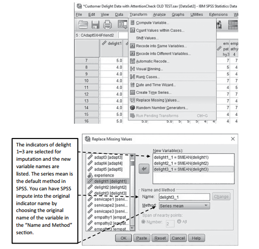
Figure 2.6  Replacing Missing Values in SPSS

It is a very similar method to impute using the linear interpolation method. After select- ing the “Transform” and “Replace Missing Values” options again, you need to select each indicator for imputation. As stated earlier, the default method is series mean, but another option under the “Name and Method” section is linear interpolation. You will need to highlight each indicator (individually), change the method to “Linear interpolation”, and then hit the “Change” button. Make sure to hit the “Change” button for each indicator. You will also see that SPSS will try to create a new column for the imputed indicator. In the example below, you will see that the indicator delight2 is (by default) being changed to delight2_1. If you do not want another column for the imputed data and simply want to keep your existing labels, you just need to change the name back to the original. In the example in Figure 2.7, delight1 is being imputed with a linear interpolation (listed as LINT), and I am keeping the same name which tells AMOS to impute the missing values in the existing column.

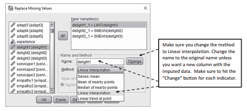
Figure 2.7  Replacing Missing Values With Linear Interpolation

Once you have made your changes and hit the “OK” button at the bottom, SPSS will impute the missing data and will give you an output of how many values were imputed. Take note in the SPSS data file that all the imputed columns (even if you kept the same name) will now be moved to the very last set of columns.

The last two imputation methods of regression imputation and full information maxi- mum likelihood will be addressed using the AMOS program. It is much easier to address these methods in AMOS than in SPSS. In Chapter 10, I go into detail on how to address regression imputation and full information maximum likelihood with the AMOS program (page 314).

Source: Thakkar, J.J. (2020). “Procedural Steps in Structural Equation Modelling”. In: Structural Equation Modelling. Studies in Systems, Decision and Control, vol 285. Springer, Singapore.