Using Specification Search to Perform Exploratory Factor Analysis in SEM

In Chapter 5, I explained how to use the specification search tool to trim a model.The specifi- cation search tool can also be used to perform an exploratory factor analysis (EFA). An EFA, as its name suggests, is an exploratory or investigative attempt to understand the factor structure of your constructs and if your indicators are loading on their appropriate factor. Unlike a con- firmatory factor analysis (CFA), each construct/factor has a relationship to every indicator in the analysis.The goal of this test is to assure that your indicators are loading on their appropri- ate construct and not on another construct in the potential model.

With many of the examples in this book, we have talked about how customers’ feelings of delight will lead to positive word of mouth about the experience. Let’s say we wanted to per- form an EFA on these two constructs. Both constructs had three observed indicators that were designed to measure the unobserved construct.The first step in testing this with the specifica- tion search function is to draw the constructs in the AMOS graphics window along with the indicators and error terms. We should have two unobserved constructs reflecting six indica- tors each. Both unobservable constructs will have a relationship to every indicator. Unlike a CFA, we do not need to set the metric, so no path from the unobservable construct to an indicator will be constrained to 1. All indicators are freely measured in this test. Saying that, we do have to set the variance for each unobservable construct to 1. This is done in order to estimate the potential different paths in the model. If we did not do this, the model would be considered under-identified. Lastly, we will still covary all unobservables in the model because they are considered independent variables. To see the standardized regression estimates, you need to go into the Analysis Properties window and select the standardized regression weight option. Do not select any other option in the Analysis Properties window, or it could create a conflict that will not display the factor loadings. See Figure 10.42 for a view of what the model should look like before using the specification search function.

Figure 10.42 Exploratory Factor Analysis Model in AMOS

After forming the model, we are ready to use the specification search function. After, we click the specification search icon   , the following window will appear (Figure 10.43).

Figure 10.43  Specification Search Window in AMOS

The first icon in this window  is the optional path function. Once you click this but- ton, you can then choose which paths in the model are optional. The optional paths function means AMOS will run numerous possible models with and without the path included. With an EFA, we will select all paths to the indicators in the model and make them optional. We initially drew a path to every indicator from an unobservable construct, and now we will see which paths are statistically necessary or important in understanding the factor structure of our model. When you select each path or single headed arrow in the model, the color of the path will change. All optional paths will show up in the model as pink.

After selecting the optional paths in the model, you are ready to run the specification search analysis by pressing the triangle button . The specification search function will then start analyzing all possible combinations of the model with the optional relationships.

The results will initially show you all the possible combinations. In this example, the speci- fication search function produced 112 different possible models. Many of the models pro- duced are inadmissible or unidentified. To find the best models produced from the analysis, you need to select the fit indices at the top. This will show you the best-fitting model first and then rank order the next best-fitting models. If I click on the chi-square/degrees of freedom heading (c/df), you can see that model 72 is listed as the best-fitting model (Fig- ure 10.44). To see model 72, you just need to double click on the model number on the left-hand side. This will show you the paths that are included/removed in the model to produce this result.

The problem you can run into is that the fit indices might actually say different models are the “best” model.The chi-square/degrees of freedom note that model 72 is the best, whereas if you click on the BIC index, we see that model 52 is the best. So how do we know which model is the best one?Which model should we use when different fit indices are suggesting different options?

Figure 10.44  Comparison of Best-Fitting Model Across Different Indices

Let’s look at both models in the AMOS graphics window to give us a better understanding on which one is more appropriate to use. Before we go into the AMOS graphics window, we need to see the parameter estimates for each model. To do this, we need to select the “Show Parameter” icon  and then double click into the model we want to view. If we double click into model 72, we see that the Positive Word of Mouth and Customer Delight indicators are strongly loading on their respective construct, but we have two additional paths included. One path is from Word of Mouth to delight3, but the loading is very weak (.08) and is not considered an acceptable factor loading. We also have a path from Customer Delight to WOM2, but again, the path is loading at an unacceptable level (−.07). We see from this model that our indicators for each construct are strongly loading on their respective factor. There is some cross loading, but it appears to be rather weak and not a huge concern.

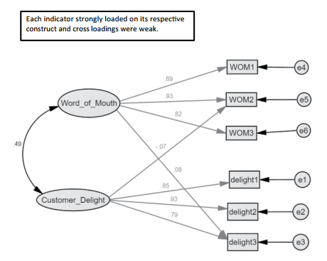
Figure 10.45 Model 72 From the Specification Search Window

Let’s now look at model 52 and see if we get a similar or different pattern of results with our indicator loadings. See Figure 10.46.

Figure 10.46 Model 52 From the Specification Search Window

With model 52, there are no cross loadings, and the only paths included in the model are from the construct of Customer Delight to its three indicators and from Positive Word of Mouth to its three indicators.The regression weights are all strong, giving initial support that all the construct’s indicators are loading on their appropriate construct.

While we have initial confirmation that our indicators are loading on our constructs,AMOS will allow us to plot/graph these results in order to see what is the most appropriate number of optional relationships. In the icon window of the specification search window is the “Plot” option. Clicking on that button    will pop up a second window with the results plotted. The plot window gives you the option of using a scree plot, a “Best fit” plot, and a scatter plot. It will also plot the results based on the different fit indices. The plots will show how much change took place on the y-axis compared to the number of different parameters estimated on the x-axis. The bottom of the screen will also show you fit values, but that information does not help in determining the appropriate model because different models will show very little difference in those values.

Of the plot model options, I find the scree plot to be most useful because it will give a clear picture on what is the optimal number of parameters to be estimated in a model. The scatter plot will give you the frequency of parameters chosen, but this is not that helpful.The “Best fit” plot method does not tell us much more than which model has the best model fit, which we can get without the plot. Let’s look at the scree plot for the chi-square/degrees of freedom index.

Figure 10.47 Scree Plot Based on Chi-Square/DF

The results show us that 13 parameters have the highest change in chi-square/degrees of freedom.When we move to a 14th parameter, the change in chi-square/degrees of freedom is substantial, and any additional parameters added are not really contributing to further expla- nation. If you click into the dot on the 13th parameter, it will give us the model number. In this example, the model number listed is model 52 that just had the three paths from Customer Delight to its indicators and the three paths from Positive Word of Mouth to its indicators. If we look at the results for the BIC index, we find similar results, where after the 13th param- eter the line abruptly drops and then levels off in regards to how much is being explained with the addition of each parameter estimate.

Across all our analyses, it appears a 13-parameter estimate is the most appropriate, which corresponds to model 52.This EFA gives strong support that our indicators are loading on the appropriate constructs. One caveat with using the specification search function is that it will allow only 30 optional arrows. If you want to run an EFA with numerous constructs at once, other statistical options may be better suited.

Figure 10.48 Scree Plot Based on BIC

Source: Thakkar, J.J. (2020). “Procedural Steps in Structural Equation Modelling”. In: Structural Equation Modelling. Studies in Systems, Decision and Control, vol 285. Springer, Singapore.