Measurement Model Invariance Across Groups in SEM Model

Up to this point, we have discussed performing a CFA with a single group. With SEM requir- ing a large sample size, it is pretty common to collect data from two different methods such as online and face-to-face surveys. You will also come across instances where you are surveying two different groups but still trying to use the same measures for each group. A measurement model invariance test is often required in those occurrences. This test is done to determine if the factor loadings of indicators in a CFA do not differ across groups.You will most often see this test performed (and required by reviewers) when you have to survey two groups and your survey items are slightly altered because of the group dynamics. An example would be if you were asking first-time customers and repeat customers the same questions but needed to make sure that the meaning of the indicators have not changed now that one group has more experi- ence with the service. A measurement model invariance test determines if your indicators are actually measuring the same thing across groups. If lack of measurement invariance is found, this indicates that the meaning of the unobservable construct is shifting across groups or possibly over time. Ultimately, you are seeing if your factor structure of your CFA is equivalent across groups.

There are five potential invariance tests to assess if you have differences in your indicators across groups. The first test that needs to be performed is called configural invariance. This initial test will examine if the overall structure of your measurement model is equivalent across groups. In essence, you are assessing the extent to which the same number of factors best represent the data for both groups. To accomplish this, you need to set up a two group analysis, which will examine if model fit is established across the groups. If strong model fit is present across both groups, then you can say with confidence that the data is invariant across the groups from a configural or structural perspective.

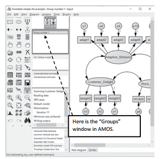
Figure 4.21 Groups Window on Graphics Page

Let’s look at how to set up a multi-group analysis and test for configural invariance. Refer- ring back to our original example, we now want to see if first-time customers are different from repeat customers.The first step is to go to the “Groups” area in AMOS. If no groups are specified, AMOS will default to one group and call it “Group number 1”. You will need to double click into “Group number 1” to bring up the “Manage Groups” window.

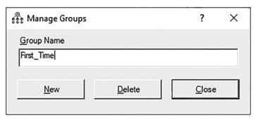
Figure 4.22  Manage Groups Pop-Up Window

(You can also access the “Manage Groups” window by going to the “Analyze” menu at the top of AMOS and then select Manage Groups). In the Manage Groups window, change the name of the group to whatever you desire. I am calling the first group “First_Time” to rep- resent the first-time customers. To create a second group, you need to hit the “New” button on the bottom of the Manage Groups window.This will form a new group (AMOS will call it Group 2 by default) and you should change the name to represent the second group. I’ll call the second group “Repeat”. After forming the groups, you need to tell AMOS where the data is for each group. Select the data file icon and then select the first group “First_Time”. Next, you can click the file name button and read the data file in for the first group. If the data for the second group is in a separate file, then you will click the second group “Repeat” and perform the same process of reading the data file into the group. If the groups are in the same data file, you will read in the same data file for each group, then you will need to hit the “Grouping Variable” button. This will ask what variable name the group distinction is in your data. Next, you need to click the “Group Value” button, and this is where you can note which value corresponds to which group. For instance, I have a column in the “Customer Delight Data” called “experience” which lists if the customer was a first-time or repeat cus- tomer. Customers who are new customers are listed as a “2” and customers who are repeat customers are a “1”.

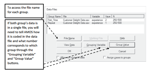
Figure 4.23 Data Files for Multiple Groups

After reading in the data for each group, you will need to uniquely label every parameter in your CFA for each group.You can imagine what a pain this would be to do this individually, but AMOS has a function that will do it for you. Hit the button (Multiple Group Analysis). Once you select this button, the following pop-up window will appear (See Figure 4.24).You can go ahead and hit “OK”. It is just stating that it is going to label every parameter and suggest potential model comparisons across the groups.

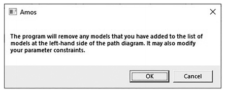
Figure 4.24 Multiple Group Warning Message

The next window that will appear is the multiple group “Models” window. Since you just requested both groups’ parameters to be labeled, AMOS will provide an unconstrained model where no parameters are constrained across the groups. It will also provide you with up to 8 constrained models. The first one is a measurement weights comparison where AMOS will constrain the measurement weights (factor loadings) for each group to be equal. Subsequent models can constrain structural weights, covariances, and errors. In a measurement model invariance test of a CFA, AMOS will propose three constrained models. I usually just hit “OK” here and let AMOS give me the models whether I will specifically use them or not.You do have the option of unchecking the boxes for a specific model if you do not want to see a specific aspect of the model constrained.

Figure 4.25 Models for Multigroup Comparison

After hitting “OK” you can go back to the main window and see on the left-hand side your groups (First_Time and Repeat). Right below that will be the unconstrained model along with all the constrained models. See Figure 4.26 for an example of what your model should look like for running the analysis. Note, if you ask AMOS to label all your parameters, it will use the letter “a” for factor loadings, “v” for error terms, and “ccc” for covariances.

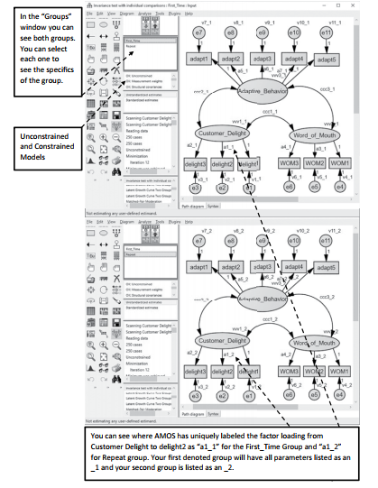
Figure 4.26 Labeling Parameters across the Groups

After labeling your groups and setting up your models, click the run analysis button  and then let’s look at the output.

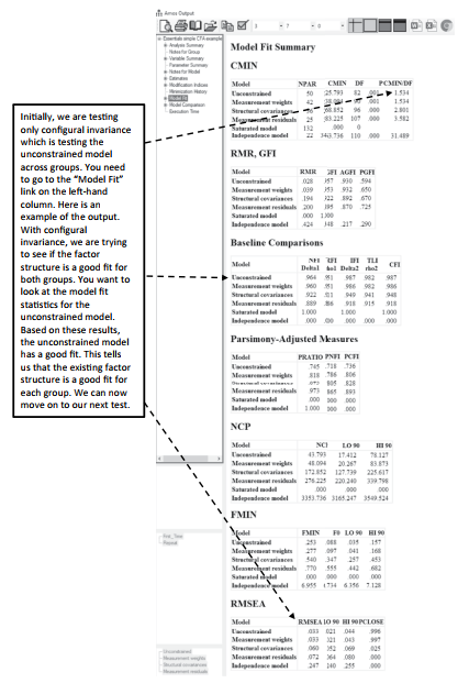
Figure 4.27 Model Fit with Multiple Group Analysis

The next model you want to assess is the metric invariance. (This is usually what most review- ers are concerned with in assessing invariance between groups.) Metric invariance establishes the equivalence of the basic “meaning” of the construct via the factor loadings across the groups. In essence, are your indicators measuring the same thing across the groups? With this multi-group analysis, you will constrain the factor loadings for each group to be equal. You will then look at the change in chi-square (from the unconstrained model) to the constrained model of factor loadings across the groups to see if there is a significant difference. If it is significant, then the meaning of your unobservable constructs is different across groups (You want non-significance here.) On the upside, once you have tested the configural invariance, it is a pretty easy process to find the metric invariance. Going back to the main graphics page in AMOS, we have already set up the two group analysis. We have also requested a constrained model where the factor loadings are constrained across the groups. In the model window, you will see it listed as “Measurement weights”.

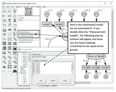
Figure 4.28  Measurement Invariance Constraints

Let’s run the analysis again     and return to the output. To assess metric invariance, you need to go to the “Model Comparison” link on the left-hand side of the output. The model comparison output compares the unconstrained model to all the constrained models you requested. For the metric invariance test, we are concerned only about the difference between the unconstrained and constrained measurement weights model.You can see below that once we constrained the 8 factor loadings across the groups and compared it to the unconstrained model, there was a non-significant difference in the chi-square value. Just to clarify, we had 11 total factor loadings but 3 are constrained to 1 in order to set the metric. Thus, only 8 factor loadings are freely estimated.

Figure 4.29 Model Comparison of Constraint Models

For many research studies, this is as far as you need to go. In some instances, further invari- ance testing is beneficial. There are three more potential tests for invariance that build off the metric invariance test.With each test, more and more constraints are added to the constraint model. These tests are run the same way as the metric invariance test, except they are listed as different models in AMOS.

1. Scalar invariance—this is where you constrain factor loadings and measurement intercepts (means) and compare this to the unconstrained In AMOS, that constrained model is called “Measurement intercepts”.
2. Factor variance invariance—this test constrains factor loadings, covariances, and vari- ances of the constructs across groups. This constrained model is called “Structural covariance”.
3. Error variance invariance—this is the most restrictive model; it constrains factor loadings, covariance, variances in the construct, and also error terms of indicators. In AMOS, this is referred to as the “Measurement Residuals” model comparison. It is highly unlikely to get a non-significant finding with this test especially if you have a lot of indicators in your model

Again, with any of these tests, you are trying to determine if a significant chi-square difference exists between the unconstrained and constrained models.The goal is to have a non-significant finding, noting that the measurement properties do not differ across the groups.

Source: Thakkar, J.J. (2020). “Procedural Steps in Structural Equation Modelling”. In: Structural Equation Modelling. Studies in Systems, Decision and Control, vol 285. Springer, Singapore.