Path Analysis in SEM Model

So far, we have talked only about the measurement model; now let’s talk about the struc- tural model.The structural model’s focus is on examining the relationships between constructs. Hence, we will look at how independent constructs influence dependent constructs or, in more complex models, how dependent variables influence other dependent variables. The first type of structural model we will examine is called a path analysis. In a path analysis, you are assessing only relationships between constructs (no measurement model items included). It is inappropriate to examine a path analysis until you have performed a measurement model analysis to determine if your measures are valid. Once the measurement model has been established, you can form composite variables for each construct. A path analysis examines the structural relationships between composite variables. Refer to Chapter 4 on how to form composite variables in SPSS.

Adding to our existing example, let’s say we have a simple model where we want to test if “Adaptive Behavior” and another construct called “Servicescape” directly influence percep- tions of Customer Delight. Just to clarify, Servicescape refers to customers’ perceptions about the built environment in which the service takes place, which could include atmos- phere, furniture, and other things related to the environment such as displays, colors, etc. From the Customer Delight construct, let’s explore if it has a relationship to Positive Word of Mouth (WOM) and another construct called “Tolerance to Future Failures”.The Tolerance to Future Failures construct is how likely a customer is to be tolerant to a service failure in the future.

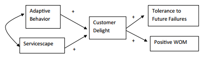
Figure 5.1  Structural Model With Composite Variables

After forming composite variables of each construct and saving the file in SPSS, you will need to read in the revised data file to AMOS. By forming a composite of a construct’s mul- tiple indicators, you have now graphically changed the construct from being a “circle” to a “square”. In essence, you have made the construct an observable. So in a path model, we will be using only squares to graphically represent the constructs.The next thing you need to do is drag in the composite constructs from the variable view to the work area.

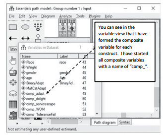
Figure 5.2 Composite Variables Used in Path Analysis

Next, you will have to add directional arrows to denote a relationship. You also need to let all the independent variables covary. In this model, comp_adapt and comp_servicescape are allowed to covary. Lastly, you need to add an error term to all dependent variables.

Make sure to label each error term as well. See Figure 5.3 of a path model in graphical form in AMOS.

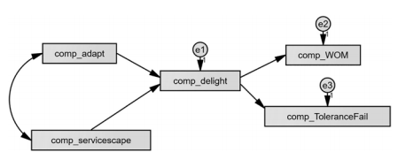
Figure 5.3 Path Model Drawn in AMOS

After forming the model, you will need to run the analysis . Make sure the “Models” window says “OK” and the computational summary window lists the chi-square value and degrees of freedom. If this is present, then you can go to the output and see your results.

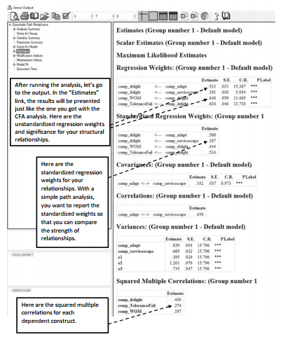
Figure 5.4 Estimates Output for Path Model

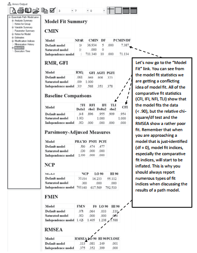
Figure 5.5 Model Fit Indices for Path Model

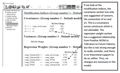
Figure 5.6 Modification Indices for Path Model

Looking at the overall results of our path model test, it appears that both constructs of Adaptive Behavior and Servicescape have a relationship to Customer Delight. The standard- ized regression weights tell us that Adaptive Behavior had a relatively stronger influence on Customer Delight (.568) compared to Servicescape (.187). The influence of Customer Delight on Positive Word of Mouth and Tolerance to Future Failures was also significant. Again, examining the standardized regression weights lets us see that Customer Delight had a stronger relative influence on Tolerance to Future Failures (.524) than on Positive WOM (.444), though both were significant.

One thing to take notice in a SEM model is whether the regression weights are positive or negative. In our example, all of the relationships are positive, which means the depend- ent construct is being positively influenced. Based on our results when Customer Delight increases, you will also see increases in an evaluation of PositiveWOM and Tolerance to Future Failures. If the regression weights were negative, that means the dependent variable is being weakened. So, if the relationship from Customer Delight to Positive WOM was negative, this would indicate that when Customer Delight evaluations increase, Positive WOM evaluations would decrease. In essence, a positive influence means that both your constructs in the rela- tionship are moving/changing in the same direction, whereas a negative influence means your constructs in the relationship are moving in opposite directions.

The squared multiple correlation (R2) for Customer Delight was .450, with the other dependent variables of Tolerance to Failure (.274) and Positive Word of Mouth (.197) showing an acceptable level of variance being explained. Unlike a CFA, there is no set or suggested criteria necessary to be explained with the squared multiple correlation values of the overall construct. These R2 values are based on the structural relationships and exhibit how much of the variance in the dependent variable is explained by the antecedent relation- ships of other variables. The R2 values of a dependent variable is influenced by how many antecedent relationships are present. In our example, Positive Word of Mouth has an influ- ence only from Customer Delight, and the R2 value of Positive Word of Mouth is how much of the variance is being explained by Customer Delight. With new and hard-to-capture concepts, having a R2 of 30% might be really good while having a R2 of 30% might be quite inadequate with a well-established construct that has numerous antecedent relationships included in the model.

The overall results for our path model in regard to model fit is a little troubling. One of the biggest drawbacks to using a path model is that you are not accounting for measurement error, which could explain some of the variance in your model. When a composite variable is formed, all the unexplained error in the measurement items are lumped together, which makes it hard to explain the variance in a model (thus having a weaker model fit). With few degrees of freedom, some model fit indices will be inflated, while others such RMSEA and relative chi-square/df test are more true to assessing how the model fits the data. Though using a path model is easy and efficient, it has issues in assessing model fit. Using a path model is very similar to other statistical techniques (e.g., PROCESS) that use composite variables, but many of those other techniques do not even assess model fit. In my opinion, if you are going to use SEM for your research, it is always better to use a full structural model that models not only measurement items but also structural relationships. More to come in this chapter about how to set up a full structural model in AMOS.

Source: Thakkar, J.J. (2020). “Procedural Steps in Structural Equation Modelling”. In: Structural Equation Modelling. Studies in Systems, Decision and Control, vol 285. Springer, Singapore.