1. INTRODUCTION
In chapters 1 to 4, attention has been focused on the difficulties inherent in formulating agreements which permit specialisation and exchange to occur, when information is not ‘public’; that is, costlessly and equally available to everyone. Specialisation permits people to concentrate on those tasks in which they have a comparative advantage (Chapter 1), and it also has more dynamic effects. As Adam Smith1 noted, specialisation results in the acquisition of enhanced levels of skill in particular operations as experience accumulates, it may permit the introduction of specialised machinery as various activities are broken down into basic components, and it may reduce the time which would otherwise be spent transferring attention from one job to the next.2 If ‘many hands make light work’ however, they may also give rise to new problems. A person who ‘saunters a little’ between tasks will at least face the costs of that sauntering if he or she is responsible for all stages in the production process. Much of Chapter 4 was devoted to the analysis of situations in which specialisation results in Adam Smith’s ‘sauntering’ turning into Alchian and Demsetz’s ‘shirking’ as people attempt to transfer the costs of their wavering attention on to others. Clearly, Smith, in his example of pin making, was considering a case of division of labour which, we may infer, he did not expect would encounter substantial coordination and policing costs. In general, however, costs of coordination and policing are not negligible (Chapter 2) and the firm itself can be seen as a response to them. These costs underlie the saying that ‘too many cooks spoil the broth’, as well as the often heard remark ‘if you want a job done properly you must do it yourself’.
The tension between the advantages of ‘specialisation’ and the costs of policing and monitoring (the advantages of ‘integration’) is a leitmotif which returns constantly in the theory of the firm. Already in Chapter 4 we have seen how different types of firm represent compromise solutions to the conflicting requirements of specialisation and incentives. In the classical proprietorship, the tasks of capitalist, monitor and risk bearer are ‘integrated’ and the problem of managerial incentives thereby mitigated. The partnership and, even more, the joint-stock company permit the ‘disintegration’ of these functions and hence the potential advantages which may accrue from exchange – a specialised management and widely spread risks – but the problem of policing and incentives is more pronounced.
In this chapter our objective is to consider the contractual problem faced by principal and agent in greater analytical detail. This will help to clarify the nature of the trade-off between risk-sharing benefits and effort incentives, and will provide a useful framework for rationalising various contractual arrangements which are observed in practice. At the outset, it is necessary to remember that the economist uses the word ‘agent’ in a much looser sense than does the lawyer. For the lawyer, an agent is ‘a person invested with a legal power to alter the principal’s legal relations with third parties’.3 Thus two partners are one another’s agents in a strict legal sense, since each can bind the other in contractual arrangements with third parties. The economist, however, is, for once, more in line with common usage in seeing the agent as a person who is employed to undertake some activity on behalf of someone else (the principal). This will cover cases of agency in the strict sense, but will also include other cases in which the same or similar incentive problems arise, although the legal term ‘agent’ would not be accurate.4
2. OBSERVABILITY AND THE SHARECROPPER
As we have seen in chapter 2, a principal-agent relation exists when one party (the agent) agrees to act on behalf of another party (the principal). (For the sake of convenience we will take the principal agent, and workers in this chapter to be male.) The problem then exists of devising a ‘contract’ which provides incentives for the agent to work in ways which benefit the principal. Let π be the final outcome of the agent’s activities, and let e represent his level of effort. Sharecropping represents the most commonly used illustrative case for discussing incentive contracts, with the landlord as the ‘principal’ and the sharecropper as his ‘agent’ (in the loose rather than the legal sense of these terms). In this case, π might represent the volume of the crop finally harvested (say bushels of wheat), while e would represent the input of the sharecropper’s time and skill. Now suppose that the final outcome is deterministically related to the sharecropper’s effort
Assuming that both sharecropper and landlord can observe the final outcome and that this outcome is conceptually simple enough to appear in a contract, it is clear that there is no reason for the landlord to monitor effort. The contract merely has to stipulate the outcome desired (say π ), and the payment to be made when it is achieved. Under these circumstances, perfect knowledge of the outcome gives us perfect information about the effort expended, and the result is a contract which is not a ‘sharecropping’ arrangement at all but simply a paid worker contract. The worker receives a specified reward upon completing the job he was hired to do. There is no incentive problem.
A case more germane to the problem of incentives occurs when the outcome depends not only on the labourer’s effort but also upon other chance factors. In the agricultural example, the harvest may depend upon climatic conditions as well as work effort. Thus we might write
![]()
where θ represents the ‘state of the world’. For example, θ might measure ‘inches of rainfall’ or ‘hours of sunshine’ or ‘average temperature in July’ and so forth. Any contract will now involve the sharing of risk in addition to the provision of incentives. Consider, once more, the paid worker contract which depends only on the achievement of a target outcome π. The labourer is unlikely to accept such an arrangement since it exposes him to considerable risk. The most careful husbandry could be powerless against adverse weather conditions and the labourer, if he is risk averse, will prefer that some account is taken either of his effort level, or of the state of the world prevailing. Clearly, however, the prospect of including e or θ in a contract depends upon whether or not they are ‘observable’. Suppose, first of all, that 0 can easily be verified by both parties. It follows, once more, that observation of the labourer’s effort is unnecessary to provide incentives, and that a preferred distribution of risk can be achieved without confronting the shirking problem.
From (5.2) both landlord and labourer will be able to work out the result (π) of a given amount of effort (e) in different states of the world (θ). The labourer’s reward (A) can therefore be made to depend upon both outcome and state of the world: A = A(π,θ). If the landlord receives an amount (P) which depends only on the state of the world P(θ), the labourer’s return would be given by
![]()
In other words, the labourer would pay to the landlord an amount P(θ) which depended on the weather, and would keep the rest of the harvest for himself. The results of additional effort always accrue to the labourer, so that no incentive problem arises, while the characteristics of P(θ) enable risks to be shared between landlord and labourer in any way desired. Such arrangements typify the ‘sharecropping’ contract. If, for example, P(θ) were a constant P’, so that the labourer paid the same amount to the landlord in every state of the world, the labourer would effectively be bearing the entire risk and insuring the landlord against the vagaries of the weather. On the other hand, the landlord’s share P(θ) could be so arranged that the remainder left for the labourer is always the same, providing the labourer puts in the standard effort e’. In this case, it would be the landlord who would bear the risk and the labourer who would receive a definite predetermined return providing the standard effort e’ was forthcoming. If both landlord and labourer were risk averse, we would not expect either to bear the entire risk. Instead P(θ) would be defined so as to share risk efficiently between them. In the next section we will discuss in more detail what it means to share risk ‘efficiently’.
Specifying a mutually agreeable contract becomes more complicated when we assume that the state of the world θ is not observable by the landlord (or principal). If effort e is unobservable also, then clearly any contract must of necessity depend upon the outcome π alone. It is this case which we will discuss in detail in section 4. Even at this stage, however, the essential character of the problem can be appreciated. The unobservability of the state variable θ and effort e means that it will, in general, be impossible to achieve an ideal distribution of risk between the parties without sacrificing effort incentives. Conversely, the ‘best’ contract achievable will usually involve the sacrifice of risk-sharing benefits in the interests of providing incentives.
Consider the case in which the landlord or principal is risk neutral and the labourer or agent is risk averse. Intuitively, we have already accepted that the risk-neutral partner should ideally bear the entire risk (a proposition which we will justify in more detail in the next section). Where the state of the world 0 is observable, it has already been shown how this distribution of risk could be arranged whilst still eliciting the standard effort e’ from the labourer. The labourer would receive the same reward whatever the state of the world, but only if he exerted the standard effort. Where the contract must depend on the outcome alone, however, assuring the labourer of a given reward is to leave him with no incentive to do anything. If the principal can never form the faintest conception of how hard the agent worked, and can never become acquainted with the difficulties he encountered, these factors cannot enter the contract. In such a case, however, a promise to pay a fixed determinate sum to the agent would be to make his remuneration completely independent of effort. The labourer would receive the same number of bushels of wheat from the landlord even if his only acquaintance with the fields to be cultivated occurred as he passed through them during his daily journeys to and from the village pub. Clearly, the provision of effort incentives requires that the labourer receives a bigger payment if the harvest is big than if the harvest is small, but because the harvest depends on the chance factors θ, this implies that the labourer must shoulder some risk, even though his landlord is risk neutral and would, in conditions of ‘observability’, provide him with complete insurance.
The above paragraph suggests that information about the labourer’s effort would be valuable in enabling both parties to a contract to achieve preferred positions. If we continue to assume that θ is unobservable by the principal, some observation of the agent’s effort e might clearly benefit both parties. By checking that the labourer sowed the correct type of seed, applied the appropriate fertiliser and so forth, it would be possible to move towards the ideal distribution of risk without diminishing effort incentives. In the extreme case of perfectly observable effort, the (risk-averse) labourer would receive a payment dependent entirely on effort and would thus face no risk, while the (risk-neutral) landlord would receive the residual harvest. Monitoring will not usually be so reliable, however, and a further interesting question is whether information about effort containing errors, which are subject to a known statistical distribution, could be incorporated in a contract to the advantage of both parties. The landlord might check at random whether the labourer is actually working in the field. An unlucky labourer could find that the spot check occurred during the only five minutes he was away, and a lucky one that it occurred during the only five minutes he was there. A series of such checks will provide information which, although not perfectly accurate, nevertheless contains potentially usable information about effort. Indeed it can be shown,5 that, irrespective of the ‘noise’ associated with the information, there will always be an advantage to incorporating an informative signal into a contract if the agent is risk averse (assuming that the signal is costlessly received and that costs of writing the contract can be ignored). A more detailed illustration of what it means for a noisy signal to be ‘informative’ will be given in section 4.
In the case of a risk-neutral labourer or agent, information about effort or state of the world will be valueless. Even in conditions of complete nonobservability of effort and state, all available risk-sharing benefits can be achieved without sacrificing incentives. As we noted above, a risk-neutral labourer will shoulder the entire risk and pay a fixed fee to the landlord. Because the fee is the same whatever the state of the world that occurs, it is clearly not necessary to observe the state. Neither will observation of the agent’s effort confer any benefits, since the agent will personally face the consequences of any ‘sauntering’ and cannot unload the costs on to the landlord. In effect, the agent simply pays a fixed fee for the use of the resources owned by the landlord for a specified period of time. This will obviously avoid any dangers associated with shirking, while the risk- neutrality assumption ensures that this arrangement is compatible with the efficient distribution of risk. The next two sections illustrate some of the above results using a set of simple diagrams.
3. RISK SHARING
Consider a case in which two people (person A and person P) wish to share the risk implied by a fluctuating harvest. Suppose that the harvest or outcome can take only two values π1 and π2 with π1 > π2. For the present,
we ignore the influence of effort on the harvest and simply assume that π1 and π2 occur with probabilities p1 and P2 = (1—Pj) respectively. Each person, we assume, will be entitled to a given portion of the harvest depending on whether the harvest is good or bad. Thus,
where π1A is person A’s entitlement when the harvest is good, π2P is person P’s entitlement when the harvest is bad, and so forth. Presented with various different combinations of π1A and π2A, it is assumed, as in elementary consumer theory, that person A is capable of ranking them in a weak ordering. The outcome of this ranking process can then be illustrated on a two-dimensional diagram using indifference curves. If person A’s preferences accord with certain axioms – the von Neumann-Morgenstern axioms6 – it can be shown that a utility function for person A can be constructed UaGa) such that his preferences over risky prospects are consistent with the expected utility attached to the prospects. Indifference curves can then be thought of as lines of constant expected utility.7
The shape of A’s indifference curves will depend upon his attitude to risk. In Figure 5.1, each point G1A, π2A) represents a prospect. At point ‘a’ for example, person A has a claim or entitlement to π¡A if the harvest is good andπ2A if the harvest is bad. Since, as drawn, π¡A = π2A, this implies that, at such a point, person A would be certain of the outcome and would be bearing no risk. Given the probability of a good harvest P1, it is clear that any portfolio of claims represented by a point in the shaded set to the north-east of ‘a’ will be more preferred, and any portfolio represented by a point in the shaded set to the south-west of ‘a’ will be less preferred, than the portfolio at ‘a’. Thus, just as in conventional consumer theory, indifference curves are expected to slope downwards from left to right. The curvature properties of the indifference curves are more complex, however.
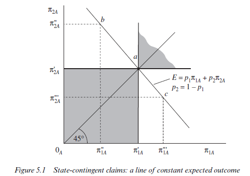
Consider the straight line p1π1A + p2π2A = E drawn through point ‘a’. By definition, all prospects along this line produce the same mathematical expectation (E) of the outcome as at point ‘a’. The slope of the line will be —(pj/p2) . Now consider a point such as b on this line. Will person A prefer ‘b’ to ‘a’ or vice versa? To answer this question, we note that a move from a to b implies a move from a riskless environment to a risky one. Person A would risk losing (k[a — ^j’A) in the event of the harvest being good, but would stand the chance of gaining (πA — π2A) in the event of the harvest being bad. However, since the expected outcome for person A is constant all along the straight line, we know that the gamble involved in moving from ‘a’ to ‘b’ is a ‘fair’ gamble. A ‘fair’ gamble is one with an expected value of zero. Person A would expect, in a mathematical sense, neither to gain nor to lose because
![]()
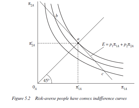
Whether person A would prefer point a or point b therefore reduces to the question of whether or not person A is prepared to take a ‘fair’ gamble. Any person who always rejects a ‘fair’ bet will prefer a to b. Such a person is ‘risk averse’. A risk-averse person will move to lower and lower levels of satisfaction (expected utility) as he or she moves away from point a in either direction along the line of constant expected outcome. Thus, the indifference curves of a risk-averse person will have the conventional convex shape familiar from elementary consumer theory. Figure 5.2 illustrates the preference map of a typical risk-averse person. An important characteristic of this preference map is that the slope of the indifference curves along the 45° line from the origin (for example, at point a) will be equal to the slope of the constant expected outcome line —(p/p2) . In other words, along the certainty line where ^1A = ^2A, each person will be prepared to exchange claims contingent upon a bad harvest for claims contingent on a good harvest in the ratio (p1/p2). This applies only to ‘points such as a’ and is therefore a proposition about limits. Although the person is risk averse, he will approach indifference between point a and a fair gamble, as the ‘stakes’ become vanishingly small. Some use will be made of this property of indifference curves in future sections.
Returning to Figure 5.1, a person who is indifferent between point a and any ‘fair’ gamble represented by another point on the constant expected outcome line (such as point b or point c) is termed ‘risk neutral’. Variability of the outcome is of no consequence for such a person. The only matter of interest is the expected value of the outcome, and all combinations of claims which yield the same mathematical expectation of the outcome are equally preferred. Thus, the indifference curves of a risk-neutral person will be straight lines with slope — (pj/p2) corresponding to lines of constant expected outcome. Maximising expected utility for this person will be the same as maximising the expected outcome. For completeness, we should add that a person who enjoys taking fair bets will prefer point b to point a, and hence a ‘risk-preferring’ person will have concave indifference curves. The case is not illustrated and no future use will be made of it.
We are now in a position to discuss the risk-sharing problem. Figure 5.3 is a ‘box diagram’ with A’s origin at the bottom left-hand corner and P’s origin at the top right-hand corner. The horizontal dimension of the box represents the total harvest if yields are good (nq) and the vertical dimension represents the total harvest if the yields are bad (^2) . Any point within the box represents a division of the total harvest between the two people in both good times and bad. Thus, point r, for example, illustrates a case in which person A has entitlements given by distance OA^JA if the harvest is good and OA^’2A if the harvest is bad; while person P has entitlements given by distance OP^P if the harvest is good and OPrn’2P if the harvest is bad. Person A’s claims plus person P’s claims sum to the total harvest.
The question now arises: does point r represent an ‘efficient’ allocation of claims between persons A and P? The answer will depend upon the preferences of the people concerned and therefore Figure 5.3 illustrates one particular case. As drawn, person A is risk averse and his convex indifference curves are drawn with respect to an origin at OA; while person P is assumed to be risk neutral and his straight line indifference curves are drawn with respect to an origin at OP. At point r, person A has utility index UA and person P has utility index Up. It is clear, however, that by exchanging claims with one another, both could be made better off; there are gains from trade to be had. Any allocation of claims represented by a point in the shaded set in Figure 5.3 will benefit at least one of the parties without harming the other; that is, they represent ‘Pareto improvements’ on point r. ‘Efficiency’ is characterised by the absence of gains from trade, as was seen in Chapter J of this book. Points of tangency between A’s indifference curves and P’s indifference curves will be efficient points. An allocation represented by a point such as s, for example, is ‘efficient’. Any move away from s must harm one or both of the parties, and therefore agreement to a move will be impossible to achieve.
As drawn in Figure 5.3, the locus of points of tangency between the indifference curves of the two parties lies along the 45° line out of A’s origin. It will be recalled that P’s indifference curves have a slope of (pj/p2) along their entire length, whilst A’s curves have a slope of (p/p2) along A’s certainty line. Thus, tangency must occur along A’s 45° line. The line between s and t represents the set of efficient allocations which are Pareto improvements on point r. By moving from point r to point t, for example, person P will be supplying person A with fair insurance. Fair insurance will benefit risk-averse A, whose utility index increases to UA. The risk taken by person P will be increased, but, for him, point t represents a fair gamble relative to point r and, being risk neutral, person P’s utility index will be the same at t as at r. A move from r to s, on the other hand, will confer all the gains from trade on person P. Person P shoulders the entire risk still, but now on somewhat ‘unfair’ terms (in an actuarial sense) relative to point r. P’s expected return and hence expected utility has increased, while A’s expected return has decreased. The fall in the expected return to A does not result in a fall in expected utility because the greater certainty of the return at s compared with r is sufficient to compensate.
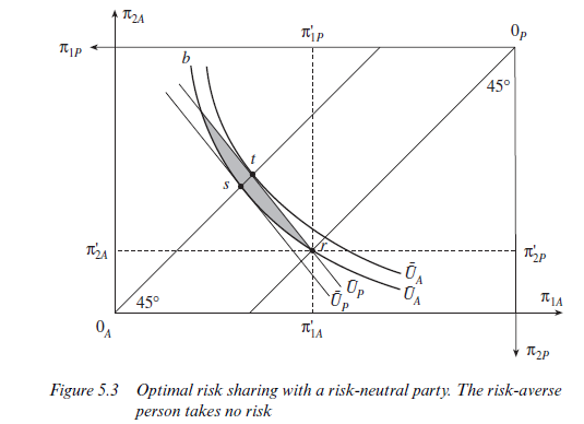
Figure 5.3 illustrates our earlier contention that efficient sharing of risk will involve a risk-neutral party providing complete insurance to the riskaverse party. Thus, in section 2, we saw that, where the state of the world 0 was observable and the effort-incentive problem could therefore be overcome, a risk-neutral landlord (employer) would take the entire risk and a risk-averse labourer (worker) would receive the same amount irrespective of whether the harvest turned out to be good or bad. Conversely, a riskneutral labourer would pay a fixed fee to a risk-averse landlord and keep the residual harvest. Where both persons are risk averse, efficient allocations of claims will be between the two 45° lines in Figure 5.3 and both parties will bear some of the risk.
4. EFFORT INCENTIVES
The principal-agent problem proper can now be considered by assuming that the probability of a good harvest is not given and unalterable, but can be influenced by the activity of the agent, person A. To keep matters as simple as it is possible to make them, let us assume that by exerting effort e, the agent is capable of changing the probability of a good harvest from pj topje wherepje>pj. The agent has a simple choice between two levels of effort, zero or e. His effort, however, is assumed to be totally unobservable by the principal, P. The final outcome or harvest can be observed by both parties, but this is all. Let the agent be risk averse and the principal be risk neutral.
Consider now the effect of effort on the agent’s indifference map. Because effort increases the probability of a good harvest to pje, the slope of all the agent’s indifference curves along A’s certainty line will steepen to —pj e/(J – pje). At any particular point on this certainty line, however, the utility index will be lower, because effort we assume is unpleasant and reduces A’s level of utility. In Figure 5.4 the indifference curve of the agent through 0 is drawn assuming no effort is exerted. The slope at 0 is — pj/(j — pj) and the utility index is UA. The curve through a is drawn on the assumption that effort eis exerted. Its slope at a is (— pje/(l — pje)) and the utility index is also UA. To show that it applies to situations where effort is being exerted, the curve is labelled UAe. Distance 0a is a measure of the ‘cost’ to A of effort e.
These two curves UAe and UA intersect at point r. A portfolio of claims represented by point r would just leave the agent indifferent between exerting effort e and not exerting any effort. At any point to the right of r and between UA and UAe, the agent would strictly prefer effort to no effort. At point s, for example, the agent will achieve a higher utility index by operating on his ‘with effort’ set of indifference curves than his ‘without effort’ set. By providing the agent with a portfolio of claims at s, we can induce the effort e. No monitoring is possible and none is required. The agent’s own self-interest will be sufficient to produce the effort. We have loaded his claims sufficiently heavily in favour of the good harvest that he has an interest in increasing the probability of this favoured event occurring; an interest powerful enough at s to overcome the disutility associated with effort.
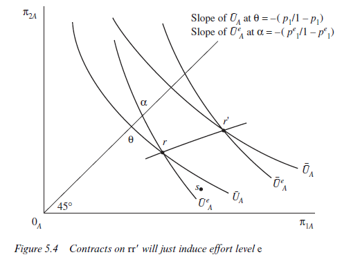
By an identical process of reasoning, we can deduce that at point r’ in Figure 5.4, the agent is also indifferent between effort and no effort. At this point, the agent’s utility index is UA> UA, whether or not effort is forthcoming. Joining up the points of intersection between ‘with effort’ and ‘without effort’ indifference curves applying to the same utility index, a locus such as rr’ is traced out. Points to the right of rr’ will induce effort e. Points to the left will not.
If it is possible to induce effort e from the agent, we still do not know whether both parties would agree to such a contract, or whether the principal would be as well off leaving the agent to relax in security at a point along his certainty line. It is this question which Figure 5.5 attempts to answer. At a point such as 0, risk would be efficiently shared between persons A and P as was shown in section 3. For effort to be forthcoming from the agent, however, a contract to the right of rr’ must be agreed. Such a contract, by increasing the probability of a good harvest topxe, will affect P’s indifference curves and not merely person A’s. P’s indifference curves will now have a slope of -pje/(1 -pxe) along their entire length. The new P indifference curve yielding the same utility index as at 0, but applying to a situation in which the agent is exerting effort, is labelled UpA. Note that it cuts P’s original indifference curve UP at π along P’s certainty line. Clearly a given point on P’s certainty line will yield the same utility index irrespective of the probability of a good harvest since, along that line, P is completely insulated from the effects of variations in the harvest.
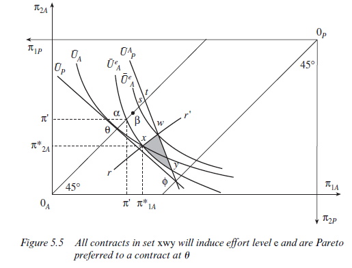
Inspection of Figure 5.5 reveals that there exists a set of contracts (the shaded set wxy) which consists of Pareto improvements on the contract at 0. Points in the set wxy are between the curves UAe and UpA, thus ensuring that the utility index of both principal and agent will be at least as great as at 0, and to the right of rr’, thus ensuring that it is the ‘with effort’ indifference curves that will be relevant and that effort e will be forthcoming from the agent. Of this set of Pareto improvements on 0, Pareto- efficient contracts will lie along the boundary between x and w. A move from point w, for example, to any other point in the shaded set will harm person A. A move from point x would harm person P. Conversely, from any point within the shaded set, it will be possible to find a point on the boundary which is preferred by both A and P.
It is important to notice that along the boundary xw, risk is not shared efficiently between principal and agent. The indifference curves of principal and agent intersect (for example, at point w) indicating that ideally there are risk-sharing benefits to be achieved by a move to A’s certainty line between s and t. These benefits are unachievable, however, because of the observability problem. Figure 5.5 therefore illustrates clearly the distinction drawn in principal-agent theory between ‘first-best’ solutions (achievable only in an ideal world of perfect observability) which lie along A’s certainty line and involve the efficient sharing of risk, and ‘Pareto-efficient contracts’ which lie along xw and are the best that can be achieved in the context of unobservable effort and state. Along xw, risk-sharing benefits are sacrificed in the interests of providing incentives. The sacrifice will be worthwhile, providing that the agent’s effort is not too costly to him for any given effect on the probability of a good harvest, or, conversely, that for any given level of the disutility of effort the effect on the probability of a good harvest is sufficiently pronounced. It is possible to envisage a case in which the distance 0a in Figure 5.5 is so large and (pxe -px) is so small that the set of Pareto improvements on 0 is empty.
Although a risk-averse agent may be made to bear some risk in the efficient contract, it is worth noting that we will never observe him bearing the entire risk. For a risk-averse agent to bear the entire risk we would have to imagine an efficient contract existing somewhere along P’s certainty line. In terms of Figure 5.5, the locus xw would have to cross P’s certainty line at some point. Risk aversion and the resulting convexity of A’s indifference curves ensure, however, that the point x must always lie to the right of UP. But points to the right of UP along P’s certainty line will leave person P with a lower utility index than at 0. Thus, there can never be an efficient contract on P’s certainty line which is Pareto preferred to 0 when A is risk averse.
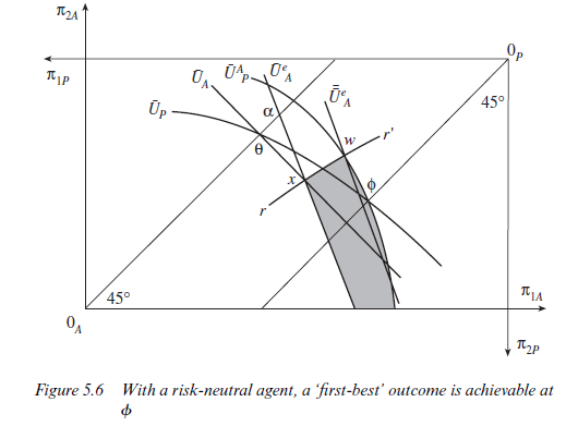
Where the agent is risk neutral, however, and the principal is risk averse it is no longer necessary to sacrifice risk-sharing benefits to achieve incentives. Incentives and risk sharing are compatible, as can be seen from Figure 5.6, and the agent will optimally bear the entire risk. The structure of the figure is the same as that of Figure 5.5. Once more contracts to the right of rr’ provide an incentive to A to exert effort level e. The set of contracts Pareto preferred to 0 is given by the shaded area. In this case, however, the boundary xw no longer represents the set of Pareto-efficient contracts. At w, for example, the agent could be made better off without harming the principal by a move to point ^, thereby achieving a more efficient distribution of risk. Points along P’s certainty line share risk efficiently and induce effort e from the agent. ‘Pareto efficient contracts’ are ‘first best’ even under conditions of unobservability. Information on the agent’s effort or on the state of the world has no value to the principal. At the agent pays a fixed fee to the principal and is entitled to keep whatever remains of the harvest.
5. INFORMATION
A risk-averse agent and a risk-neutral principal (Figure 5.5) will have to sacrifice risk-sharing benefits if effort is to be induced under conditions of ‘unobservability’. The ability to observe the agent’s effort is therefore valuable because it enables risk-sharing benefits to be captured. Information about the agent’s effort may be subject to error, however, and it is not immediately obvious whether principal and agent would both agree to use this kind of information in their contractual arrangements. As reported in section 2, abstracting from the costs of writing and enforcing an increasingly complex contract, an informative signal, no matter how noisy, can be used to increase the utility of both parties. In this section we illustrate this proposition using the simple example of principal and agent discussed in section 4.
Suppose to begin with that no information about the agent’s effort is used in the contract. Efficient contracts will then lie along the locus rr’ in Figure 5.5. Consider the efficient contract at x. As argued at length earlier, the agent at x will just be indifferent between effort and no effort. By exerting effort the agent faces one gamble and by not exerting effort he faces another (different) gamble. He is just indifferent between these two gambles. Specifically, if the agent remains idle he faces the following gamble:
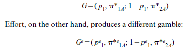
where in this case π*e1A represents the outcome π*1A bushels having exerted effort level e. From our diagram we know that for person A, GIGe, where I represents indifference.
Now let the principal (landlord) monitor the agent (labourer) through a series of spot checks mentioned in section 2. He may visit the field at random a given number of times. If the labourer is never there, the landlord will conclude (perhaps wrongly) that his effort level has been zero. Providing the labourer is there at least once, the landlord will conclude (again perhaps wrongly) that effort level e has been forthcoming. Satisfying this crude spot-check test will yield a reward of + Se and not satisfying it will incur a penalty of – 8o. Might such an arrangement be agreeable to both principal and agent?
Ignore for the present the problem of how the labourer is to know whether the landlord is telling the truth when the latter claims to have seen neither hide nor hair of the former. This is an important issue which will be taken up later in Chapter 6 on hierarchies. Assuming that the landlord monitors in the way described, the labourer will be able to calculate the probability that he is observed hard at work when in fact he has been idle, as well as the probability that he is observed to be idle when in fact he has been hard at work and so forth. Let the first subscript represent the landlord’s observation of effort and the second subscript the tenant’s actual effort. Thus let
qoe = probability that landlord observes zero effort when actual effort is e;
qee = probability that landlord observes effort e when actual effort is e;
qeo = probability that landlord observes effort e when actual effort is zero;
qoo = probability that landlord observes zero effort when actual effort is zero.
With these probabilities, we can construct a number of new gambles which we might call ‘monitoring gambles’. Consider, for example, the following prospects:
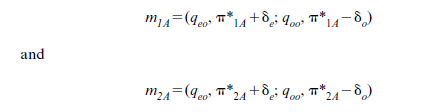
These are the gambles the labourer would face if his effort level were zero. They depend upon the harvest. If the harvest turned out to be good and the labourer had agreed to be monitored, he would then face gamble miA. Similarly, if the harvest were bad, the labourer would then face gamble m2A. By agreeing to be monitored, therefore, the idle labourer would change the original gamble G into the complex gamble Gm where
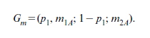
Suppose now that qoo > qeo; that is, the landlord is more likely to observe ‘correctly’ than ‘incorrectly’. If the labourer is idle, it is more likely that he will be observed as such than that he will be observed exerting effort e. This is our minimal requirement for the landlord’s monitoring to be ‘informative’. If qoo = qeo, the spot checks would produce a signal that was all ‘noise’ and no information. If qoo< qeo, the signal would be positively misleading. Further, assume that 8e < 8o.
Clearly, if qoo > qeo, and 8o >Se, gambles miA and m2A are statistically ‘unfair’. The labourer would prefer ^*A to the gamble miA, and rn*LA to the gamble m2A, assuming that he is risk averse. Thus, we deduce that the idle labourer will not want to be monitored and that he will prefer G to Gm.
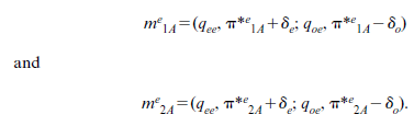
For the industrious labourer, the situation is rather different, however. He will face the ‘monitoring gambles’:
If he consents to be monitored, the original gamble Ge will change to the more complex gamble
![]()
Again, suppose that the monitoring of the landlord is ‘informative’ so that qee >qoe and that the industrious labourer is more likely to be seen as industrious than idle. Further, assume that the reward 8e and the penalty 8o are set such that 8e<8o as above, but also qee8e = qoe8o. Gambles me1A and me2A will then both be ‘fair’ gambles.
As was seen in section 3, a risk-averse labourer will reject a fair bet. However, we also saw in section 3 that as the ‘stakes’ were reduced a riskaverse person would approach indifference between taking and not taking a fair bet. People are risk neutral ‘in the limit’. Thus, we might imagine 8e and 8o being reduced in size whilst always maintaining the ratio 8e/8o = qoe/qee. In the limit, the industrious labourer will be indifferent between Gme and Ge. Because the ‘monitoring gambles’ m1A and m2A are statistically unfavourable, the idle labourer, on the other hand, will always strictly prefer G to Gm and can never be brought to indifference no matter how tiny the stakes.
At point x, therefore, we have the following results as 8e,8o tend to zero with 8e /So = qoe /qee
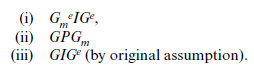
Thus, GmePGm. Without the monitor, the labourer at x is just indifferent between effort and no effort. With the monitor and an ‘informative signal’, we can construct a situation in which the labourer strictly prefers effort to no effort at x and is no worse off in his own estimation than he was in the absence of the monitor (GmeIGeIG).
Consider now how the principal is affected by these arrangements. We continue to assume that the signal is costlessly observed. Providing that the monitoring gambles me1A and me2A are ‘fair’, the risk-neutral principal will be prepared to offer them to the agent whatever the absolute sizes of 8e and 8o. Even if the principal were risk averse, we could apply the same argument used above for the agent to show that he would approach indifference as the stakes declined. Thus, in the limit, neither principal nor agent will be any worse off from a risk-bearing point of view as a result of the ‘monitoring gambles’. Work incentives, however, have changed, as we have seen, and the benefits from this enhanced work incentive can be used to increase the utility index of either the principal or agent.
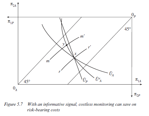
The argument is illustrated diagrammatically in Figure 5.7. The locus rr’ represents, as before, points at which the agent is indifferent between effort and no effort, when no information about effort is used in the contract. Monitoring, as described in the earlier paragraphs of this section, using noisy but informative signals, results in effort being strictly preferred by the agent at x. It will therefore be possible to find another point such as y at which the agent is once more indifferent between effort and no effort even in the context of monitoring.8 The locus of all such points might be represented by the curve mm’. At y, the utility of the industrious labourer will be the same as at x, but the utility of the landlord will be greater than at x. Monitoring, by providing a source of additional effort incentives, enables risk-sharing benefits to be achieved without reducing the amount of effort forthcoming. In effect, monitoring is being used as a substitute for a more inefficient distribution of risk as a means of inducing effort.
Source: Ricketts Martin (2002), The Economics of Business Enterprise: An Introduction to Economic Organisation and the Theory of the Firm, Edward Elgar Pub; 3rd edition.
I have not checked in here for a while as I thought it was getting boring, but the last several posts are great quality so I guess I will add you back to my daily bloglist. You deserve it my friend 🙂