Sata Example Program

1. Example Program: multicat (Plot Many Categorical Variables)

The preceding sections presented basic ideas and example short programs. In this section, we apply those ideas to a longer program that defines a new statistical procedure named multicat.

Survey research produces datasets containing many categorical variables — sometimes 100 or more. Our 2010 General Social Survey excerpt provides a smaller example with just 19 variables, most of which are categorical responses to survey questions.

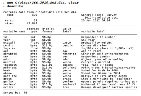
As a first step in exploring such data, or to prepare a preliminary report, we might simply construct tables showing percentage distributions for each variable. The following command would produce eight such tables, for all variables in the dataset frompolviews to evolve.

. tabl polviews – evolve

Stata provides no similarly easy way to draw and save bar charts for a variable list, however. As a programming example, this section shows a makeshift program that was written to meet that particular need when it arose during a complex survey project.

Program multicat, defined by the ado-file that follows, builds upon another user-written program named catplot, introduced in Chapter 4. catplot can draw a variety of graphs showing the distribution of a categorical variable. multicat is more specialized, producing only horizontal bar charts for percentages in each category; but this is a particularly useful format for presenting survey data. multicat adds the ability to handle a list of many variables, which catplot and other Stata graphing commands cannot do. Thus, we could ask multicat to draw bar charts of all the variables in our dataset, saving each graph individually along the way. As written, the program saves graphs both in Stata (gph) format and in one other format (emf, eps or pdf depending on the operating system), with file names based on the variable names. You could change any of these specifications by editing multicat.ado, tailoring the program to your own analytical needs.

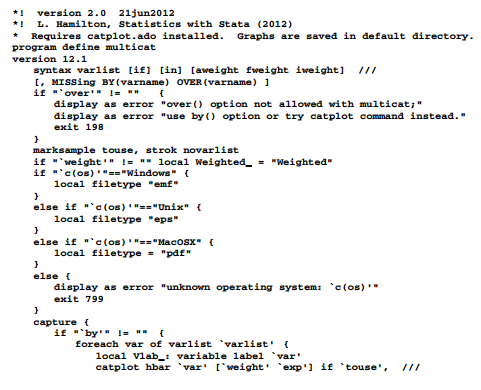
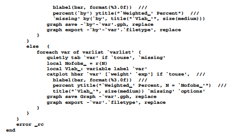
Indentation of lines has no effect on the program’s execution, but makes it easier for the programmer to read. The heart of multicat is its syntax statement, and then a foreach loop that repeatedly calls catplot for each variable in the variable list. Local macros pass information to the catplot command that actually draws the graphs. The command allows analytical weights (aweights) which have an effect here similar to that of probability weights (pweights) in a svy: tab command. It allows in or if qualifiers. Optionally we could include missing values, and use by( ) but not over( ).

The multicat program was written incrementally, beginning with a do-file named multicat.do. Starting with input components such as the syntax statement, the do-file was run to see how things worked before adding other components. Not all of the trial runs produced satisfactory results. Typing the command

. set trace on

causes Stata to display programs line-by-line as they execute, so we can see exactly where an error occurs. Later, we can turn this feature off by typing

. set trace off

Preliminary multicat.do versions contained the first line, capture program drop multicat, to discard the program from memory before defining it again. This was necessary during the writing and debugging stage, when a previous version of our program might have been incomplete or incorrect. Such lines should be deleted when the program is mature, however.

Once we believe our do-file defines a program that we will want to use again, we can create an ado-file. This is accomplished just by saving the file with an .ado extension (multicat.ado). The recommended location is in ado\personal; you might need to create this directory and
subdirectory if they do not already exist. Other locations are possible, but review the User’s Manual section on “Where does Stata look for ado-files?” before proceeding. Once this is done, we can use multicat as a regular command within Stata.

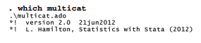
The program could be refined further to make it more flexible, elegant and user-friendly. Note the inclusion of comments stating the source and “version 2.0” in the first two lines, which both begin *! The comment refers to version 2.0 of multicat.ado, not Stata (an earlier version of multicat.ado appeared in the previous edition of this book). The Stata version suitable for running this program is specified by the version 12.1 command a few lines later. Although the *! comments do not affect how the program runs, they are visible to a which command:

2. Using multicat

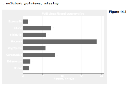
After multicat.ado has been saved (for example, in C:\ado\personal), the command multicat becomes usable as if it were an ordinary (albeit, unfinished) feature of Stata. Figure 14.1 shows responses regarding political views. Both percentages and the number of observations appear in the plot.

Survey data commonly are analyzed using probability weights and svyset data, as discussed in Chapter 4. Applying survey weights, svy: tab finds the following responses to the question about legalizing marijuana.

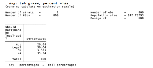
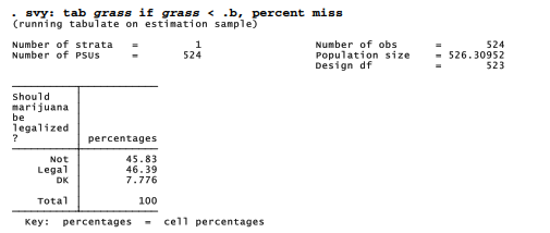
This question has two kinds of missing values. About 5% of the respondents were asked the marijuana question but said they did not know, or declined to give an answer. Their missing values have been coded .a, with value label “DK”. Another 35% in this sample were not asked the grass question. Those have been coded .b, with value label “NA”. The GSS accommodates a large number of questions by asking different questions to subsets of their sample. Analytically it makes sense for us to set aside the un-asked group and recalculate the percentages. Doing so, we find an even split: about 46% in favor and 46% opposed to legalizing marijuana, with 8% undecided.

multicat (based on catplot) does not understand svy: commands or probability weights, but analytical weights (aweights) have the same effect here. Figure 14.2 shows a multicat plot corresponding to the table above. The multicat graphic also notes the relevant sample size (524).

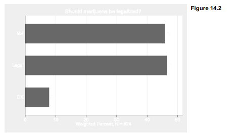
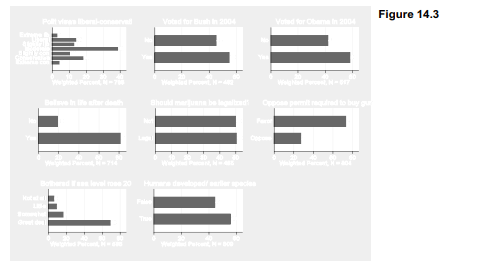
A series of many graphs like Figure 14.2, dropped into a document or slide show, could be read and annotated by the analyst for a quick presentation of results. Setting aside the complication of missing values, here is a quick example where multicat draws a set of 8 bar charts for the variables frompolviews to evolve. multicat automatically saves each graph with filenames such as

-polviews.gph. A graph combine command then fits the graphs into one image, Figure 14.3.

. multicat polviews-evolve [aw = wtssall]

. graph combine -polviews.gph -bush.gph -obama.gph

-postlife.gph -grass.gph -gunlaw.gph -sealevel.gph -evolve.gph

Survey research becomes more interesting as we start to compare subgroups. For example, the even split on legalizing marijuana looks different when broken down by gender in Figure 14.4.

This is where multicat comes into its own, offering an easy way to draw many comparison charts. The following commands draw 8 bar charts for opinions broken down by gender, then combine 4 of the separate charts into one image, Figure 14.5. We see that female respondents are more likely than males to believe in life after death (86 versus 76%), oppose legalizing
marijuana (57 versus 43%), favor gun permits (77 versus 68%) or reject evolution (49 versus 39%).

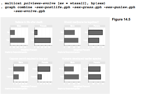
The graph combine step is used in Figures 14.3 and 14.5 for compact illustrations of what multicat is doing. In research, the actual number of graphs often exceeds what we want to crowd into one image. A multicat command could just as easily draw 100 graphs comparing survey responses by men and women, then 100 more comparing responses by education level, age group, political party, region or any other categories of interest. Most analysts will never need this particular trick, but when specialized needs arise in a project, makeshift programs of this sort could become essential.

Source: Hamilton Lawrence C. (2012), Statistics with STATA: Version 12, Cengage Learning; 8th edition.