Some elementary concepts and tools, combined with the Stata capabilities described in earlier chapters, suffice to get started.
1. Do-files
Do-files are text (ASCII) files, created by Stata’s Do-file Editor, a word processor, or any other text editor. They are typically saved with a .do extension. The file can contain any sequence of legitimate Stata commands. In Stata, typing the following command causes Stata to read filename.do and execute the commands it contains:
. do filename
Each command in filename.do, including the last, must end with a hard return, unless we have reset the delimiter through a #delimit command:
#delimit ;
This sets a semicolon as the end-of-line delimiter, so that Stata does not consider a line finished until it encounters a semicolon. Setting the semicolon as delimiter permits a single command to extend over more than one physical line. Later, we can reset “carriage return” as the usual end-of-line delimiter with another #delimit command:
#delimit cr
A typographical note: Many commands illustrated in this chapter are most likely to be used inside a do-file or ado-file, instead of being typed as a stand-alone command in the Command window. I have written such within-program commands without showing a preceding “.” prompt, as with the two #delimit examples above (but not with the do filename command, which would have been typed in the Command window as usual).
2. Ado-files
Ado (automatic do) files are ASCII files containing sequences of Stata commands, much like do-files. The difference is that we need not type do filename in order to run an ado-file. Suppose we type the command
. clear
As with any command, Stata reads this and checks whether an intrinsic command by this name exists. If a clear command does not exist as part of the base Stata executable (and, in fact, it does not), then Stata next searches in its usual “ado” directories, trying to find a file named clear.ado. If Stata finds such a file (as it should), it then executes whatever commands the file contains.
Ado-files have the extension .ado. User-written programs (written by you) commonly go in a directory named C:\ado\personal, and programs written by other Stata users typically go in C:\ado\plus. The hundreds of official Stata ado-files get installed in C:\Program Files\Stata\ado. Type sysdir to see a list of the directories Stata currently uses. Type help sysdir or help adopath for advice on changing them.
The which command reveals whether a given command really is an intrinsic, hardcoded Stata command or one defined by an ado-file; and if it is an ado-file, where that resides. For example, summarize is a built-in command, but the regress command currently is defined by an ado-file named regress.ado, updated in April 2011.
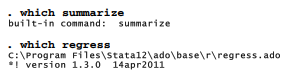
This distinction makes no difference to most users, because summarze and regress work with similar ease when called. Studying examples and borrowing code from Stata’s thousands of official ado-files can be helpful as you get started writing your own. The which output above gave the location for file regress.ado. To see its actual code, type
. viewsource regress.ado
The ado-files defining Stata estimation commands have grown noticeably more complicated- looking over the years, as they accommodate new capabilities such as svy: prefixes.
3. Programs
Both do-files and ado-files might be viewed as types of programs, but Stata uses the word “program” in a narrower sense, to mean a sequence of commands stored in memory and executed by typing a particular program name. Do-files, ado-files or commands typed interactively can define such programs. The definition begins with a statement that names the program. For example, to create a program named count5, we start with
program counts
Next should be the lines that actually define the program. Finally, we give an end command, followed by a hard return:
end
Once Stata has read the program definition commands, it retains a definition of the program in memory and will run it any time we type the program’s name as a command:
. counts
Programs effectively make new commands available within Stata, so most users do not need to know whether a given command comes from Stata itself or from an ado-file-defined program.
As we start to write a new program, we often create preliminary versions that are incomplete or unsuccessful. The program drop command provides essential help here, allowing us to clear programs from memory so that we can define a new version. For example, to clear program count5 from memory, type
. program drop counts
To clear all programs (but not the data) from memory, type . program drop _all
4. Local macros
Macros are names (up to 31 characters) that can stand for strings, program-defined numerical results or user-defined values. A local macro exists only within the program that defines it, and cannot be referred to in another program. To create a local macro named iterate, standing for the number 0, type
local iterate 0
To refer to the contents of a local macro (0 in this example), place the macro name within left and right single quotes. For example,
display ‘iterate’
0
Thus, to increase the value of iterate by one, we write
local iterate = ‘iterate’ + 1
display ‘iterate’
1
Instead of a number, the macro’s contents could be a string or list of words, such as
local islands Iceland Faroes
To see the string contents, place double quotes around the single-quoted macro name:
display “‘islands'”
Iceland laroes
We can concatenate further words or numbers, adding to the macro’s contents. For example,
local islands ‘islands’ Newfoundland Nantucket
display “‘islands'”
Iceland Faroes Newfoundland Nantucket
Type help extended fcn for information about Stata’s “extended macro functions,” which extract information from the contents of macros. For instance, we could obtain a count of words in the macro, and store this count as a new macro named howmany:
local howmany: word count ‘islands’ display ‘howmany’
4
Many other extended macro functions exist, with applications to programming.
5. Global macros
Global macros are similar to local macros, but once defined, they remain in memory and can be used by other programs for the duration of your current Stata session. To refer to a global macro’s contents, we preface the macro name with a dollar sign (instead of enclosing the name in left and right single quotes as done with local macros):
global distance = 73
display $distance * 2
146
Unless we specifically want to keep macro contents for re-use later in our session, it is better (less confusing, faster to execute, and potentially less hazardous) if we use local rather than global macros in writing programs. To drop a macro from memory, issue a macro drop command.
macro drop distance
We could also drop all macros from memory
macro drop _all
6. Scalars
Scalars can be individual numbers or strings, referenced by a name much as local macros are. To retrieve the contents, however, we do not need to enclose the scalar name in quotes. For example,
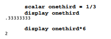
Scalars are most useful in storing numerical results from calculations, at full numerical precision. Many Stata analytical procedures retain results such as degrees of freedom, test statistics, log likelihoods, and so forth as scalars — as can be seen by typing return list or ereturn list after the analysis. The scalars, local macros, matrices and functions automatically stored by Stata programs supply building blocks that could be used within new programs.
7. Version
Stata’s capabilities have changed over the years. Consequently, programs written for an older version of Stata might not run directly under the current version. The version command works around this problem so that old programs remain usable. Once we tell Stata for what version the program was written, Stata makes the necessary adjustments and the old program can run under a new version of Stata. For example, if we begin our program with the following statement, Stata interprets all the program’s commands as it would have in Stata 9:
version 9
Typed by itself, the command version simply reports the version to which the interpreter is currently set.
8. Comments
Stata does not attempt to execute any line that begins with an asterisk. Such lines can therefore be used to insert comments and explanations into a program, or interactively during a Stata session. For example,
* This entire line is a comment.
Alternatively, we can include a comment within an executable line. The simplest way to do so is to place the comment after a double slash, // (with at least one space before the double slash). For example,
summarize logsize age // this part is the comment
A triple slash (also preceded by at least one space) indicates that what follows, to the end of the line, is a comment; but then the following physical line should be executed as a continuation of the first. For example,
summarize logsize age /// this part is the comment
educ income
will be executed as if we had typed
summarize logsize age educ income
With or without comments, a triple slash tells Stata to read the next line as a continuation of the present line. For example, the following two lines would be read as one table command, even though they are separated by a hard return.
table married sex, ///
contents(median age)
The triple slash thus provides an alternative to the #delimit ; approach described earlier, for writing program commands that are more than one physical line long.
It is also possible to include comments in the middle of a command line, bracketed by /* and */. For example,
table married sex, /* this is the comment */ contents (median age)
If one line ends with /* and the next begins with */ then Stata skips over the line break and reads both lines as a single command — another line-lengthening trick sometimes found in programs, although /// is now favored.
9. Looping
There are a number of ways to create program loops. One simple method employs the forvalues command. For example, the following program counts from 1 to 5.
* Program that counts from one to five
program counts
version 12.1
forvalues i = 1/5 {
display ‘i’
}
end
By typing these commands, we define program count5. Alternatively, we could use the Do-file Editor to save the same series of commands as an ASCII file named count5.do. Then, typing the following causes Stata to read the file:
. do counts
Either way, by defining program count5 we make this available as a new command:
. counts
1
2
3
4
5
The command
forvalues i = 1/5 {
assigns to local macro i the consecutive integers from 1 through 5. The command
display ‘i’
shows the contents of this macro. The name i is arbitrary. A slightly different notation would allow us to count from 0 to 100 by fives (0, 5, 10, …100):
forvalues j = 0(5)100 {
The steps between values need not be integers, so long as the endpoints are. To count from 4 to 5 by increments of .01 (4.00, 4.01, 4.02, …5.00), write
forvalues k = 4(.01)5 {
Any lines containing valid Stata commands, between the opening and closing curly brackets {}, will be executed repeatedly for each of the values specified. Note that apart from optional comments, nothing on that line follows the opening bracket, and the closing bracket requires a line of its own.
The foreach command takes a different approach. Instead of specifying a set of consecutive numeric values, we give a list of items for which iteration occurs. These items could be variables, files, strings, or numeric values. Type help foreach to see the syntax of this command.
forvalues and foreach create loops that repeat for a pre-specified number of times. If we want looping to continue until some other condition is met, the while command is useful. A section of program with the following general form will repeatedly execute the commands within curly brackets, so long as expression evaluates to “true”:
while expression {
command A
command B
……
}
command Z
As in previous examples, the closing bracket } should be on its own separate line, not at the end of a command line.
When expression evaluates to “false,” the looping stops and Stata goes on to execute command Z. Parallel to our previous example, here is a simple program that uses a while loop to display onscreen the iteration numbers from 1 through 6:
* Program that counts from one to six
program count6
version 12.1
local iterate = 1
while ‘iterate’ <= 6 {
display ‘iterate’
local iterate = ‘iterate’ + 1
}
end
A more substantial loop appears in the multicat.ado program described later in this chapter. The Programming Reference Manual contains more about programming loops.
If . . . else
The if and else commands tell a program to do one thing if an expression is true, and something else otherwise. They are set up as follows:
if expression {
command A
command B
…
}
else {
command Z
}
For example, the following program segment checks whether the content of local macro span is an odd number, and informs the user of the result.
if int(‘span’/2) != (‘span’ – 1)/2 {
display “span is NOT an odd number”
}
else {
display “span IS an odd number”
}
10. Arguments
Programs define new commands. In some instances (as with the earlier example, count5), we intend our command to do exactly the same thing each time it is used. Often, however, we need a command that is modified by arguments such as variable names or options. There are two ways we can tell Stata how to read and understand a command line that includes arguments. The simplest of these is the args command.
The following do-file (listresl.do) defines a program that performs a two-variable regression, and then lists the observations with the largest absolute residuals. listresl exhibits several bad habits, such as dropping variables and leaving new ones in memory, which could have unwanted side effects. It serves to illustrate the use of temporary variables, however.
- Perform simple regression and list observations with #
- largest absolute residuals.
- syntax: listres1 Yvariable Xvariable # IDvariable
capture drop program listres1
program listres1, sortpreserve
version 12.1
args Yvar Xvar number id
quietly regress ‘Yvar’ ‘Xvar’
capture drop Yhat_
capture drop Resid_
capture drop Absres_
quietly predict Yhat_
quietly predict Resid_,
resid quietly gen Absres_ = abs(Resid_)
gsort -Absres_
drop Absres_
list ‘id’ ‘Yvar’ Yhat_ Resid_ in 1/’number’
end
The line args Yvar Xvar number id tells Stata to assign arguments to four macros. These arguments could be numbers, variable names or other strings separated by spaces. The first argument becomes the contents of a local macro named Yvar, the second a local macro named Xvar, and so forth. The program then uses the contents of these macros in other commands, such as the regression:
quietly regress ‘Yvar’ ‘Xvar’
The program calculates absolute residuals (Absres), and then uses the gsort command (with minus sign before the variable name) to sort data in high-to-low order, with missing values last:
gsort -Absres_
The option sortpreserve on the command line makes this program “sort-preserving,” ensuring that the order of the observations is the same after the program runs as it was before.
Dataset Nations2.dta contains information on 194 countries, including per capita CO2 emissions (co2), per capita gross domestic product (gdp) and country name (country). We can open this file, and use it to demonstrate our new program. A do command runs do-file listres1.do, thereby defining the program and new command listresl:
. use C:\data\Nations2.dta, clear
. do C:\data\listres1
Next, we use the newly-defined listresl command, followed by its four arguments. The first argument specifies the y variable, the second x, the third how many observations to list, and the fourth gives the case identifier. In this example, our command asks for a list of observations that have the five largest absolute residuals.
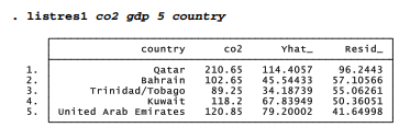
In these five oil-exporting nations, per capita CO2 emissions are much higher than predicted from GDP.
11. Syntax
The syntax command provides a more complicated but also more powerful way to read a command line. The following do-file named listres2.do is similar to our previous example, but it uses syntax instead of args.
- Perform simple or multiple regression and list
- observations with # largest absolute residuals.
- listres2 yvar xvarlist [if] [in], number(#) [id(varname)] capture drop program listres2
program listres2, sortpreserve version 12.1
syntax varlist(min=1) [if] [in], Number(integer) [Id(varlist)] marksample touse
quietly regress ‘varlist’ if ‘touse’
capture drop Yhat_
capture drop Resid_
capture drop Absres_
quietly predict Yhat_ if ‘touse’
quietly predict Resid_ if ‘touse’, resid
quietly gen Absres_ = abs(Resid_)
gsort -Absres_
drop Absres_
list ‘id’ ‘1’ Yhat_ Resid_ in 1/’number’
end
listres2 has the same purpose as the earlier listresl: it performs regression, then lists observations with the largest absolute residuals. This newer version contains several enhancements, made possible by the syntax command. It is not restricted to two-variable regression, as was listresl. listres2 will work with any number of predictor variables, including none (in which case, predicted values equal the mean ofy, and residuals are deviations from the mean). listres2 permits optional if and in qualifiers. A variable identifying the observations is optional with listres2, instead of being required as it was with listresl. For example, we could regress CO2 emissions on Gross Domestic Product and percent urban, while restricting our analysis to nations in region 2, the Americas.

The syntax line in this example illustrates some general features of the command:
syntax varlist(min=1) [if] [in], Number(integer) [Id(varlist)]
The variable list for a listres2 command is required to contain at least one variable name (varlist(min=1)). Square brackets denote optional arguments — in this example, the if and in qualifiers, and also the id( ) option. Capitalization of initial letters for the options indicates the minimum abbreviation that can be used. Because the syntax line in our example specified Number(integer) Id(varlist), an actual command could be written:
. listres2 co2 gdp, number(6) id(country)
or, equivalently,
. listres2 co2 gdp, n(6) i(country)
The contents of local macro number must be an integer, and id one or more variable names.
This example also illustrates the marksample command, which marks the subsample (as qualified by if and in) to be used in subsequent analyses.
The syntax of syntax is outlined in the Programming Manual. Experimentation and studying other programs help in gaining fluency with this command.
Source: Hamilton Lawrence C. (2012), Statistics with STATA: Version 12, Cengage Learning; 8th edition.
As I website possessor I believe the content matter here is rattling great , appreciate it for your hard work. You should keep it up forever! Best of luck.