Since 1972, the General Social Survey (Davis et al. 2005) has tracked U.S. public opinion through a series of annual or biannual surveys, and made the data available for teaching and research. Dataset GSS_2010_SwS contains a small subset of variables and observations from the 2010 survey, including background variables along with answers to questions about voting, marijuana, gun control, climate change and evolution. The General Social Survey website provides detailed information about this rich data resource (http://www3.norc.org/GSS+Website/).

The GSS question about evolution will be our focus in this section. This question, one item in a science-literacy quiz, asks whether it is true or false that
Human beings, as we know them today, developed from earlier species of animals.
This question invokes individual beliefs as well as science knowledge. About 55% of the respondents said the statement is true.
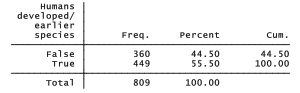
Non-missing values for evolve were the criterion for selecting this subset of 809 GSS respondents. “False” responses to evolve have been recoded as 0 and “True” as 1. The question of survey weighting, a complicated issue with multilevel modeling and not yet resolved for Stata’s mixed-effects logit command xtmelogit, is not addressed here.
Research commonly finds that science literacy increases with education, and also is related to other background factors. In the case of evolve, we might expect some connection with political outlook as well. A simple logit regression confirms these hypotheses, finding that male, better educated, and politically moderate to liberal respondents more often believe in human evolution.

Apart from such individual-level predictors of evolution beliefs, there might be a region-level component as well. Controversies about teaching evolution in schools have been most prominent in the South. Consistent with this impression, a chi-squared test of the GSS data finds significant differences between U.S. census divisions. Acceptance of evolution is highest (89%) among respondents in New England — the states of Connecticut, Maine, Massachusetts, New Hampshire, Rhode Island and Vermont. It is lowest (36%) among those in the E South Central division — the states of Alabama, Kentucky, Mississippi and Tennessee. The Pacific and W South Central divisions are second highest and second lowest, respectively.

We could add census division to our regression as a set of indicator variables for divisions 2 through 9, each contrasted with division 1, New England.

Coefficients on the indicator variables give the shift in ^-intercept for that division in comparison with New England. All of these coefficients are negative because the log odds of accepting evolution are lower in other divisions than in New England. As expected, the difference is greatest for division 6, E South Central. Only division 9, Pacific, is not significantly different from New England. Net of these region-level effects, all of the individual- level predictors also show significant effects in the expected directions.
An indicator-variable approach works here because we have only 9 clusters (census divisions), and are testing simple hypotheses about shifts in ^-intercepts. With more clusters or more complicated hypotheses, a mixed-effects approach could be more practical. For example, we might include random intercepts for each census division in a mixed-effects logit regression model, as follows. The syntax of xtmelogit resembles that of xtmixed.

Random intercepts in the output above exhibit significant variation, judging by a likelihood- ratio test versus an ordinary logistic regression (p = .0167), or by the standard deviation of random intercepts (.3376) being more than twice its standard error (.1559). The next commands estimate values for these random intercepts through predict, then make a table showing them by cendiv. Consistent with the earlier chi-squared and indicator-variable analyses, we see positive random y-intercepts (shifting the total effect up) for the New England and Pacific divisions, but negative random y-intercepts (shifting the total effect down) for E South Central and W South Central divisions.

So by any method, we see a robust pattern of regional differences in evolution beliefs, even controlling for individual factors. Mixed-effects modeling allows us to go farther by testing more detailed ideas about regional differences. The literature identifies education as a key influence on evolution and other science beliefs. Do the effects of education differ by census division? We could test this by including both random intercepts and slopes:
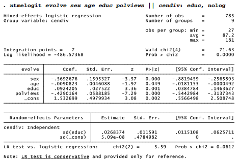
The standard deviation of random slopes on education is more than twice its standard error, suggesting significant regional variation. The standard deviation of random intercepts, on the other hand, is near zero — meaning there is no place-to-place variation in this term. A simpler model omitting the random intercepts through a nocons option gives an identical log likelihood.

The simplified random-slope model above implies that education has different effects on evolution beliefs in different parts of the country. To see what those effects are, we can predict the random slopes, creating a new variable named raneduc. Total effects of educ equal these random effects plus the fixed effect given by the coefficient _b[educ]. A constant “variable” named fixeduc is generated to display the fixed effects in a table, and a new variable toteduc gives the total effects of education, or the slope on educ within each census division.

From the table, we can confirm that the total education effects equal fixed plus random effects. Figure 13.10 visualizes these total effects.

We see that education has a positive effect on the log odds of accepting evolution across all census divisions. Education effects are much stronger, however, among respondents in New England or Pacific states compared with the E or W South Central.
Source: Hamilton Lawrence C. (2012), Statistics with STATA: Version 12, Cengage Learning; 8th edition.
Hello there, You have done a great job. I will certainly digg it and personally suggest to my friends. I am sure they will be benefited from this website.