Exponential and Weibull Regression by using Stata

Cox regression estimates the baseline survivor function empirically without reference to any theoretical distribution. Several alternative parametric approaches begin instead from assumptions that survival times do follow a known theoretical distribution. Possible distribution families include the exponential, Weibull, lognormal, log-logistic, Gompertz or generalized gamma. Models based on any of these can be fit through the streg command. Such models have the same general form as Cox regression (equations [10.2] and [10.3]), but define the baseline hazard h ₀ (t) differently. Two examples appear in this section.

If failures occur independently, with a constant hazard, then survival times follow an exponential distribution and could be analyzed by exponential regression. Constant hazard means that the individuals studied do not “age,” in the sense that they are no more or less likely to fail late in the period of observation than they were at its start. Over the long term, this assumption seems unjustified for machines or living organisms, but it might approximately hold if the period of observation covers a relatively small fraction of their life spans. An exponential model implies that logarithms of the survivor function, ln(5(t)), are linearly related to t.

A second common parametric approach, Weibull regression, is based on the more general Weibull distribution. This does not require failure rates to remain constant, but allows them to increase or decrease smoothly over time. The Weibull model implies that ln(-ln(5(t))) is a linear function of ln(t).

Graphs provide a useful diagnostic for the appropriateness of exponential or Weibull models. For example, returning to aids.dta, we construct a graph (Figure 10.6) of ln(S(t)) versus time, after first generating Kaplan-Meier estimates of the survivor function S(t). The y-axis labels in Figure 10.6 are given a fixed two-digit, one-decimal display format (%2.1f) and oriented horizontally, to improve their readability.

The pattern in Figure 10.6 appears somewhat linear, encouraging us to try an exponential regression:

The hazard ratio (1.074) and standard error (.035) estimated by this exponential regression do not greatly differ from their counterparts (1.085 and .038) in our earlier Cox regression. The similarity reflects the degree of correspondence between empirical hazard function and the
constant hazard implied by an exponential distribution. According to this exponential model, the hazard of an HIV-positive individual developing AIDS increases about 7.4% with each year of age.

After streg, the stcurve command draws a graph of the models’ cumulative hazard, survival or hazard functions. By default, stcurve draws these curves holding all x variables in the model at their means. We can specify other x values by using the at( ) option. The individuals in aids.dta ranged from 26 to 50 years old. We could graph the survival function at age = 26 by issuing a command such as

. stcurve, surviv at(age = 26)

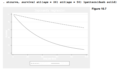
A more interesting graph uses the at1( ) and at2( ) options to show the survival curve at two different sets of x values, such as the low and high extremes of age:

Instead of the exponential distribution, streg can also fit survival models based on the Weibull distribution. A Weibull distribution might appear curvilinear in a plot of ln(5(t)) versus t, but it should be linear in a plot of ln(-ln(5(f))) versus ln(f), such as Figure 10.8. An exponential distribution, on the other hand, will appear linear in both plots and have a slope equal to 1 in the ln(-ln(5(f))) versus ln(t) plot. In fact, the data points in Figure 10.8 are not far from a line with slope 1, suggesting that our previous exponential model is adequate.

Although we do not need the additional complexity of a Weibull model with these data, results are given below for illustration.

The Weibull regression obtains a hazard ratio estimate (1.079) intermediate between our previous Cox and exponential results. The most noticeable difference from those earlier models
is the presence of three new lines at the bottom of the table. These refer to the Weibull distribution shape parameterp. Ap value of 1 corresponds to an exponential model: the hazard does not change with time. p > 1 indicates that the hazard increases with time; p < 1 indicates that the hazard decreases. A 95% confidence interval for p ranges from .79 to 1.62, so we have no reason to reject an exponential (p = 1) model here. Different, but mathematically equivalent, parameterizations of the Weibull model focus on ln(p), p or 1/p, so Stata provides all three. stcurve draws survival, hazard, or cumulative hazard functions after streg, dist(weibull) just as it does after streg, dist(exponential) or other streg models.

Exponential or Weibull regression is preferable to Cox regression when survival times actually follow an exponential or Weibull distribution. When they do not, these models are misspecified and can yield misleading results. Cox regression, which makes no a priori assumptions about distribution shape, remains useful in a wider variety of situations.

In addition to exponential and Weibull models, streg can fit models based on the Gompertz, lognormal, log-logistic or generalized gamma distributions. Type help streg or consult the Survival Analysis and Epidemiological Tables Reference Manual for syntax and a list of options.

Source: Hamilton Lawrence C. (2012), Statistics with STATA: Version 12, Cengage Learning; 8th edition.