Specifying the Phenomenon or System to be Modeled in the Research

Models can be defined as abstract representations of real phenomena. They represent the components of the phenomena studied as much as they do the interrelationships among these components. Identifying the phenomenon or system to be modeled is a three-step process. The first step is to determine its components. The interrelationships between these components must then be specified. Finally, because these models are representations, the researcher will want to formalize them through a graphic or mathematical description of the components and their presumed interrelations. Most often, a model will be rep­resented by circles, rectangles or squares linked by arrows, curves, lines, etc.

1. Components of a Model

A model, in its most simple form (a relationship of cause and effect between two variables), essentially comprises two types of variables with different func­tions: independent variables (also called explanatory or exogenous variables) and dependent variables (also called variables to be explained, or endogenous variables). In this causal relationship, the independent variable represents the cause and its effect is measured on the dependent variable.

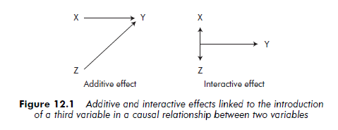
Quite often, the phenomenon being studied includes more elements than simply an independent variable and a dependent variable. A single dependent variable is liable to have multiple causes. Several independent variables may explain one dependent variable. These variables are considered as causes in the same way as the initial causal variable, and produce an additive effect. They are an addition to the model and explain the dependent variable.

The introduction of new variables within a simple causal relationship between two independent and dependent variables may also produce an inter­active effect. In this case, the dependent variable is influenced by two causal variables whose effect can only be seen if these two associated variables intervene at the same time.

Figure 12.1 schematizes the additive and interactive effects linked to the introduction of a third variable, Z, into a simple causal relationship between two variables, X and Y.

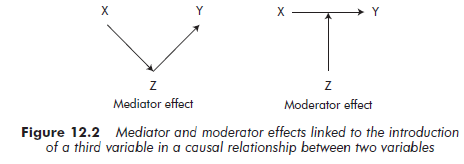
Finally, variables can intervene in the direct causal relationship between the dependent variable or variables and the independent variable. These variables, described as intervenors, take two forms: mediator or moderator.

When the effect of the independent variable X on the dependent variable Y is measured by the intermediary of a third variable Z, we call this third variable a mediator. The association or causality observed between X and Y results from the fact that X influences Z, which in turn influences Y (Baron and Kenny, 1986).

A moderator variable modifies the intensity (increasing or decreasing) and/or the sign of the relationship between independent and dependent vari­ables (Sharma et al., 1981). The moderator variable enables researchers to iden­tify when certain effects are produced and then to break down a population into subpopulations, according to whether the measured effect is present or not. Figure 12.2 schematizes the mediator and moderator effects relative to the introduction of a third variable in the relationship between independent and dependent variables.

To move from a phenomenon to a model, it is not enough just to identify the different variables involved. One must also determine the status of these vari­ables: dependent, independent (with an additive or interactive effect), modera­tor or mediator.

2. Relationships

Three types of relationship are possible between two of a phenomenon’s vari­ables (Davis, 1985). The first two are causal, while the third involves simple association:

• The first possibility is a simple causal relationship between the two vari­ables: X => Y (X influences Y, but Y does not influence X).

Example: A simple causal relationship

Introducing the theory of the ecology of populations to explain organizational iner­tia and organizational change, Hannan and Freeman (1984) postulate that selection mechanisms favor companies whose structures are inert. They present organiza­tional inertia as the result of natural selection mechanisms. The variable ‘natural selection’ therefore acts on the variable ‘organizational inertia’.

• The second relationship involves a reciprocal influence between two vari­ables: X => Y => X (X influences Y, which in turn influences X).

Example: A reciprocal causal relationship

Many authors refer to the level of an organization’s performance as a factor that pro­vokes change. They consider that weak performance tends to push organizations into engaging in strategic change. However, others point out that it is important to take the reciprocal effect into account. According to Romanelli and Tushman (1986), organizations improve their performance because they know how to make timely changes in their action plan. There is, therefore, a reciprocal influence between per­formance and change, which can be translated as follows: weak performance pushes companies to change and such change enables performance to be improved. ^[1]

• The third relationship demonstrates that an association exists between thetwo variables. However, it is not possible to determine  which causes the other: X <=> Y (X relates to Y and Y to X).

Once the nature of the relationship has been determined, it is important to establish its sign. This is either:

• positive, with X and Y varying in the same direction
• or negative, with X and Y varying in opposite directions.

In a causal relationship, the sign translates as follows. It is positive when an increase (or reduction) in X leads to an increase (or decrease) in Y and it is nega­tive when an increase (or decrease) in X leads to a decrease (or increase) in Y. In the case of an association between two variables, X and Y, the sign of the rela­tionship is positive when X and Y are high or low at the same time and nega­tive when X is high and Y is low and vice versa.

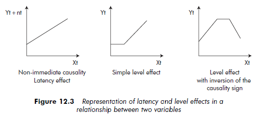
In a relationship between two variables, causality is not always immediate. Indeed, there can be a latent effect – a period during which the effect of a variable is awaited. This effect is particularly significant when researchers use correla­tion to test relationships between two temporal sets. They need to determine what period of time elapses between the cause and effect, and to separate the two series accordingly to conduct this test. It is possible that the relationship or causality will only be effective below a certain level. As long as the value of X remains below this level, X has no influence on Y (or there is no relationship between X and Y). When the value of X goes beyond this level, then X has an influence on Y (or there is a relationship between the two variables X and Y). An effect related to level may also influence the relationship’s sign. For example, below a certain level, the relationship is positive. Once this level has been attained, the sign is inverted and becomes negative. Figure 12.3 schematizes these different effects.

Whatever the nature or sign of the relationship, causality can only be speci­fied in two ways: deductively, starting from theory, or inductively, by observa­tion. Researchers must begin with the hypothesis of a causal relationship between two variables, either based on theory or because observation is tend­ing to reveal it. Only then should they evaluate and test the relationship, either quantitatively or qualitatively.

3. Formal Representation

Models are usually represented in the form of diagrams. This formalization responds, above all, to the need to communicate information. A drawing can be much clearer and easier to understand than a lengthy verbal or written descrip­tion, not least when the model is complex (that is, contains several variables and interrelations).

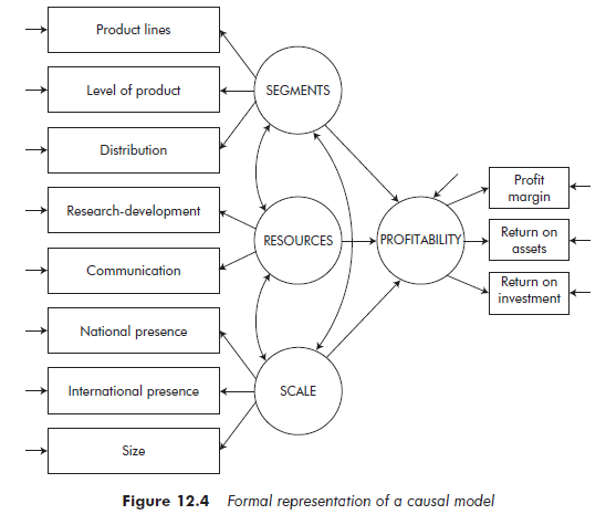
Over the years, a diagrammatic convention has developed from ‘path analy­sis’ or ‘path modeling’, (see Section 3). According to this convention, concepts or variables that cannot be directly observed (also called latent variables, concepts or constructs) are represented by circles or ellipses. Variables that can be directly observed (manifest and observed variables, and measurement variables or indi­cators) are represented by squares or rectangles. Causal relationships are indica­ted by tipped arrows, with the arrowhead indicating the direction of causality. Reciprocal causality between two variables or concepts is indicated by two arrows going in opposite directions. Simple associations (correlations or covariance) between variables or concepts are indicated by curves without arrowheads, or two arrowheads going in opposite directions at the two ends of the same curve. A curve that turns back on one variable or concept indicates variance (covariance of an element with itself). Arrows without origin indicate errors or residues.

Figure 12.4 is an example of a formal representation of a model examining the relationship between strategy and performance. In this example, ‘product lines’ or ‘profit margin’ are directly observable variables, and ‘scale’ or ‘profitability’ are concepts (that is, variables that are not directly observable). The hypothesis is that three causal relationships exist between the concepts of ‘segments’, ‘resources’ and ‘scale’, on the one hand, and that of ‘profitability’ on the other. There is also assumed to be an association relationship between the three concepts ‘segments’, ‘resources’ and ‘scale’. Finally, all the directly observable variables contain terms of error as well as the concept of ‘profitability’.

There is scope for the notion of a model to be very widely accepted in quan­titative research. Many statistical methods aim to measure causal relationships between variables by using a model to indicate the relationship system. This is often expressed by equations predicting the dependent or explained variables that are to be explained by other variables (known as independent or explana­tory variables). An example is linear regression or analysis of variance.

These explanatory methods are particular examples of more general tech­niques through which causal relationship networks can be examined (Hoyle, 1995). These techniques are known by various names; such as ‘path analysis’ or ‘path modeling’, which we have already mentioned, ‘causal model analysis’ or ‘causal modeling’, ‘structural equations analysis’ or ‘structural equation model­ing’ and ‘latent variable analysis of structural equations’. Some of them even just carry the name of a computer program, such as LISREL, PLS or AMOS. In this chapter, we have decided to use the term ‘causal model’ to indicate these techniques for examining causal relationship networks.

Causal models do not necessarily have to be represented graphically. They can also be represented mathematically. As a rule, causal models are expressed in the form of equations. These are often matrix equations, in which case the general notation takes the following form:

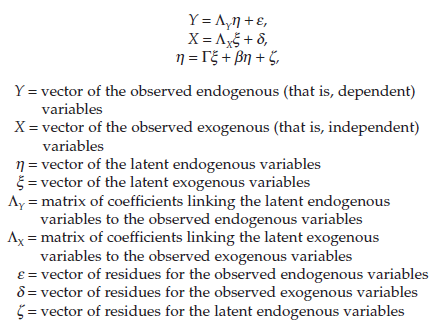
r = the matrix of causal relationships between the latent exogenous and the endogenous variables

β = the matrix of causal relationships between the latent endogenous variables.

Causal models are interesting not only because they produced the conven­tion for formally representing phenomena or modeling systems. They are also the most successful technique for modeling causal relationships quantitatively, illustrating the quantitative process that takes place at each stage.

Source: Thietart Raymond-Alain et al. (2001), Doing Management Research: A Comprehensive Guide, SAGE Publications Ltd; 1 edition.