This tutorial shows how to compute new variables in SPSS using formulas and built-in functions. The data file in example is available to download here.
1. Computing Variables
Sometimes you may need to compute a new variable based on existing information (from other variables) in your data. For example, you may want to:
- Convert the units of a variable from feet to meters
- Use a subject’s height and weight to compute their BMI
- Compute a subscale score from items on a survey
- Apply a computation conditionally, so that a new variable is only computed for cases where certain conditions are met
In this tutorial, we’ll discuss how to compute variables in SPSS using numeric expressions, built-in functions, and conditional logic.
To compute a new variable, click Transform > Compute Variable.
![]()
The Compute Variable window will open where you will specify how to calculate your new variable.
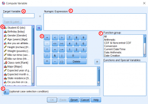
A- Target Variable: The name of the new variable that will be created during the computation. Simply type a name for the new variable in the text field. Once a variable is entered here, you can click on “Type & Label” to assign a variable type and give it a label. The default type for new variables is numeric.
B- The left column lists all of the variables in your dataset. You can use this menu to add variables into a computation: either double-click on a variable to add it to the Numeric Expression field, or select the variable(s) that will be used in your computation and click the arrow to move them to the Numeric Expression text field (C).
C- Numeric Expression: Specify how to compute the new variable by writing a numeric expression. This expression must include one or more variables from your dataset, and can use arithmetic or functions.
When writing an expression in the Compute Variables dialog window:
- SPSS is not case-sensitive with respect to variable names.
- When specifying the formula for a new variable, you have to option to include or not include spaces after the commas that go between arguments in a function.
- Do not put a period at the end of the expression you enter into the Numeric Expression box.
D- The center of the window includes a collection of arithmetic operators, Boolean operators, and numeric characters, which you can use to specify how your new variable will be calculated. There are many kinds of calculations you can specify by selecting a variable (or multiple variables) from the left column, moving them to the center text field, and using the blue buttons to specify values (e.g., “1”) and operations (e.g., +, *, /).
E- If: The If option allows you to specify the conditions under which your computation will be applied.
F- Function group: You can also use the built-in functions in the Function group list on the right-hand side of the window. The function group contains many useful, common functions that may be used for calculating values for new variables (e.g., mean, logarithm). To find a specific function, simply click one of the function groups in the Function Group list. You will now see a list of functions that belong to that function group in the Functions and Special Variables area. If you click on a specific function, a description of that function will appear in the text field to the left.
Click If (indicated by letter E in the above image) to open the Compute Variable: If Cases window.
1- The left column displays all of the variables in your dataset. You will use one or more variables to define the conditions under which your computation should be applied to the data.
2- The default specification is to Include all cases. To specify the conditions under which your computation should be applied, however, you will need to click Include if case satisfies condition. This will allow you to specify the conditions under which the computation will be applied to your data.
3- The center of the dialog box includes a collection of arithmetic operators, Boolean operators, and numeric characters, which you can use to specify the conditions under which your recode will be applied to the data. There are many kinds of conditions you can specify by selecting a variable (or multiple variables) from the left column, moving them to the center text field, and using the blue buttons to specify values (e.g., “1”) and operations (e.g., +, *, /). You can also use the built-in functions in the Function Group list under the right column.
After you are finished defining the conditions under which your computation will be applied to the data, click Continue. Note that when you specify a condition in the Compute Variable: If Cases window, the computation will only be performed on the cases meeting the specified condition. If a case does not meet that condition, it will be assigned a missing value for the new variable.
2. Computing Variables using Syntax
You do not necessarily need to use the Compute Variables dialog window in order to compute variables or generate syntax. You can write your own syntax expressions to compute variables (and it is often faster and more convenient to do so!) Syntax expressions can be executed by opening a new Syntax file (File > New > Syntax), entering the commands in the Syntax window, and then pressing the Run button.
The general form of the syntax for computing a new (numeric) variable is:
COMPUTE NewVariableName = formula.
EXECUTE.
The first line gives the COMPUTE command, which specifies the name of the new variable on the left side of the equals sign, and its formula on the right side of the equals sign. The formula on the right side of the equals sign corresponds to what you would enter in the Numeric Expression field in the Compute Variables dialog window.
The EXECUTE command on the second line is what actually carries out the computation and adds the variable to the active dataset. (If you have tried to run COMPUTE syntax but do not see variables added to your dataset and do not also see error or warning messages in the Output Viewer, you may have forgotten to run the EXECUTE statement.)
Notice how each line of syntax ends in a period.
It’s also possible to use COMPUTE syntax to compute or transform string variables (i.e., variables containing characters other than numbers). To compute string variables, the general syntax is virtually identical. However, with string variables, you must first “declare” a new variable as a string variable before you can define it using a COMPUTE statement:
STRING  NewVariableName (A20).
COMPUTE NewVariableName = formula.
EXECUTE.
On the first line, STRING statement declares the new variable’s name (NewVariableName) and its format (A20) of a new string variable. Note that the format must be put inside parentheses. The format specification for strings will always start with the letter A, followed by a number giving the “width” of the string (the maximum number of characters that variable can contain). In this case, the new variable will have a width of 20, so data values can contain up to 20 characters. When declaring a new string variable, you should take care to set the width of the string to be wide enough so that your data values aren’t accidentally cut short. On the second line, the COMPUTE statement gives the actual formula for the variable declared in the STRING statement. On the third line, the EXECUTE command tells SPSS to carry out the computation.
In general, when writing an expression or formula using COMPUTE syntax:
- SPSS is not case-sensitive with respect to variable names.
- When specifying the formula for a new variable, you have to option to include or not include spaces around the equals sign and/or after the commas between arguments in a function.
- A period goes at the end of the COMPUTE statement, after the end of the formula.
3. Example: Computing a New Variable Using Arithmetic
Now we will use what we have learned throughout this tutorial to demonstrate how to compute a new variable. In this example, we wish to compute BMI for the respondents in our sample. The height (in inches) and weight (in pounds) of the respondents were observed; so to compute BMI, we want to plug those values into the formula

Using the Compute Variables Dialog Window
- Click Transform > Compute Variable.
- In the Target Variable field, type a name for the new variable that will be computed. Let’s call our new variable BMI.
- In the Numeric Expression field, type the following expression:
(Weight*703)/(Height**2)(Alternatively, you can double-click on the variable names in the left column to move them to the Numeric Expression field, and then write the expression around them.) This expression says that the new variable will be calculated as variable Weight multiplied by 703, divided by the square of variable Height.
- Click OK to complete the computation.
- Finally, let’s make sure that a new variable called BMI was successfully created.
- We can find the new variable in the last column in Data View or in the last row of Variable View. If you do not see the new variable, the computation was unsuccessful.
- We can check the syntax that was executed by looking at the log in the Output Viewer window. If there was an error in how the computation was specified, the log in the Output Viewer will often show an error message.
- It is also useful to explore whether the computation you specified was applied correctly to the data. You can spot-check the computation by viewing your data in the Data View tab. To check that the new variable computed correctly, you can manually calculate the BMI for a few cases in your dataset just to spot-check that the computation worked correctly.
Using Syntax
Alternatively, you can produce the same result by opening a syntax window (File > New > Syntax) and executing the following code:
COMPUTE BMI=(Weight*703)/(Height**2).
EXECUTE.
This syntax can be generated automatically by following the dialog window steps above and clicking Paste instead of OK.
4. Example: Computing a New Variable Using a Built-In Function
Using the Compute Variables Dialog Window
Let’s instead try computing the average test score using the built-in mean function.
- Click Transform > Compute Variable.
- In the Target Variable area, type a name for the new variable that will be computed; let’s call the new variable AverageScore2.
- In the Function group list, click All.
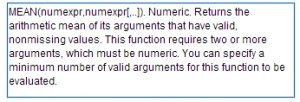
- In the Functions and Special Variables list, scroll down until you find “Mean”, then click on it. A description of this function will appear in the text box to the left. In this example, the description reads:

- Double-click “Mean” in the Functions and Special Values list. When you do this, the text
MEAN(?,?)should appear in the Numeric Expression field. - Now add each of the variables (i.e., English, Reading, Math, Writing) to the numeric expression by double-clicking on the variable names in the left list. The variable names should be separated by commas, and all of the variable names should remain inside the parentheses.
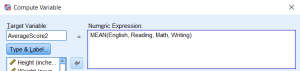
- Your final numeric expression should appear as
MEAN(English, Reading, Math, Writing). This says that the new variable, AverageScore2, will be calculated as the mean of the four test scores. (Using spaces after the commas is optional, but recommended, since it is easier to read.) - Click OK to complete the computation and apply the changes to the data.
- Finally, let’s make sure that a new variable called AverageScore2 was successfully created.
- We can find the new variable in the last column in Data View or in the last row of Variable View. If you do not see the new variable in the Variable View, the computation was unsuccessful. Additionally, if you see the new column in the Data View but every row has a missing value, there was an issue with your computation.
- We can check the syntax that was executed by looking at the log in the Output Viewer window. If there was an error in how the computation was specified, the log in the Output Viewer will often show an error message.
- It is also useful to explore whether the computation you specified was applied correctly to the data. You can spot-check the computation by viewing your data in the Data View tab. To check that the new variable computed correctly, you can manually calculate the averages for a few cases in your dataset just to spot-check that the computation worked correctly.

Using Syntax
Alternatively, you can produce the same result by opening a syntax window (File > New > Syntax) and executing the following code:
COMPUTE AverageScore2=MEAN(English, Reading, Math, Writing).
EXECUTE.
This syntax can be generated automatically by following the dialog window steps above and clicking Paste instead of OK.
5. Example: Referring to a Range of Variables in a Function
Notice that in the sample dataset, the test score variables in the sample dataset are all next to each other. In the previous example, we explicitly specified all four test score variables in the MEAN function. But what if there had been ten or twenty test score variables? It would take much longer to manually enter all twenty variable names.
What if we wanted to refer to the entire range of test score variables, beginning with English and ending with Writing, without having to type out each variable’s name?
When using SPSS’s special built-in functions, you can refer to a range of variables by using the statement TO. Let’s repeat the previous example and show how the TO statement is used to refer to a range of variables inside a function.
This method is dependent on the positions of the variables in the dataset. If the variables are not in sequential order, this method may not work correctly.
Using the Compute Variables Dialog Window
- Click Transform > Compute Variable.
- In the Target Variable area, type a name for the new variable that will be computed; let’s call the new variable AverageScore3.
- In the Function group list, click All.
- In the Functions and Special Variables list, scroll down until you find “Mean”, then click on it.
- Double-click “Mean” under in the Functions and Special Values list. The basic setup for using this function will now appear in the Numeric Expression field.
- Inside the MEAN function, change the arguments to
English TO Writing. Your final numeric expression should appear asMEAN(English TO Writing)The final expression indicates that the new variable, AverageScore3, will be calculated as the average of all the variables between English and Writing in the dataset.
- Click OK to complete the computation.
- Finally, let’s make sure that a new variable called AverageScore3 was successfully created.
- We can find the new variable in the last column in Data View or in the last row of Variable View. If you do not see the new variable, the computation was unsuccessful.
- We can check the syntax that was executed by looking at the log in the Output Viewer window. If there was an error in how the computation was specified, the log in the Output Viewer will often show an error message.
- It is also useful to explore whether the computation you specified was applied correctly to the data. You can spot-check the computation by viewing your data in the Data View tab. To check that the new variable computed correctly, you can manually calculate the averages for a few cases in your dataset just to spot-check that the computation worked correctly.
If you’ve already verified the computation for AverageScore2, then you should be able to verify that AverageScore2 and AverageScore3 are identical.
Using Syntax
Alternatively, you can produce the same result by opening a syntax window (File > New > Syntax) and executing the following code:
COMPUTE AverageScore3=MEAN(English TO Writing).
EXECUTE.
This syntax can be generated automatically by following the dialog window steps above and clicking Paste instead of OK.
6. Example: Computing Subscale Scores when Some Values Missing
In the previous examples, we did not talk about what happens when one or more of the variables has missing values for a given case. In fact, if there is a missing value for one or more of the input variables, SPSS assigns the new variable a missing value. That is, there must be valid values for each input variable in order for the computation to work. This is called listwise exclusion.
Listwise exclusion can end up throwing out a lot of data, especially if you are computing a subscale from many variables.
In SPSS, you can modify any function that takes a list of variables as arguments using the .n suffix, where n is an integer indicating how many nonmissing values a given case must have. As long as a case has at least n valid values, the computation will be carried out using just the valid values.
In the previous example, we used the built-in MEAN() function to compute the average of the four placement test scores. If we change the formula for AverageScore3 to MEAN.3(English TO Writing), then any case with three or more nonmissing values will have a successful, nonmissing value for AverageScore3. (Stated another way, a given case could have at most one missing test score and still be OK.)
Alternatively, using the formula MEAN.2(English TO Writing) would require that two or more of the test score variables have valid values (i.e., a given case could have at most two missing test scores).
Syntax
If you click Paste after revising the formula, the following syntax will be written to the syntax editor window:
COMPUTE AverageScore3=MEAN.3(English TO Writing).
EXECUTE.
7. Example: Computing a New Indicator from Several Existing Indicators
A common scenario on health questionnaires is to have multiple questions about risk factors for a certain disease. These questions may originally be coded as 0 (absent) and 1 (present); or 0 (no) and 1 (yes). For example, on a questionnaire about ADHD, we may ask three questions about whether an individual’s biological parents or siblings have been diagnosed with ADHD:
- Has your biological mother been diagnosed with ADHD?
- Has your biological father been diagnosed with ADHD?
- If you have siblings or half-siblings, has at least one of them been diagnosed with ADHD?
Suppose we want to only have a single indicator variable, where 0 = does not have any risk factors, and 1 = has one or more risk factors. The function ANY() is a convenient way to compute this indicator. The ANY function is designed to return the following:
- ANY(value, var1, var2, var3, …) = 1 if at least one of var1, var2, var3, … equals value
- ANY(value, var1, var2, var3, …) = 0 if all of the nonmissing values of var1, var2, var3, … do not equal value
- ANY(value, var1, var2, var3, …) = missing if there are missing values for each of var1, var2, var3, …
The application we will demonstrate is intended to be used when you want to check for one specific value across many variables.
For this example, we will use this tiny dataset. Each variable represents a “yes/no” question, with 1=No, 2=Yes.
You can copy, paste, and execute the following syntax to generate this dataset in SPSS, or you can download the linked SPSS datafile below.
DATA LIST FREE (",") / q1 to q3.
BEGIN DATA.
1,2,2,
2,1,,
1,1,1,
2,,1,
1,,2,
1,1,,
1,2,1,
2,,2,
1,1,2,
,,,
1,,,
,,2,
2,2,2,
END DATA.
VALUE LABELS q1 to q3 1 'No' 2 'Yes'.
-
Example Data for Computing Variable using ANY() Function (*.sav)
Using the Compute Variables Dialog Window
- Click Transform > Compute Variable.
- In the Target Variable area, type a name for the new variable that will be computed; let’s call the new variable any_yes.
- In the Numeric Expression box, enter the expression
ANY(2, q1 TO q3)
Do not put a period at the end of the expression.
This expression tells SPSS to look for instances of the value 2 (Yes) across variables q1, q2, and q3. - Click OK to complete the computation.
- Finally, let’s make sure that a new variable called any_yes was successfully created.
- We can find the new variable in the last column in Data View or in the last row of Variable View. If you do not see the new variable, the computation was unsuccessful.
- We can check the syntax that was executed by looking at the log in the Output Viewer window. If there was an error in how the computation was specified, the log in the Output Viewer will often show an error message.
- It is also useful to explore whether the computation you specified was applied correctly to the data. You can spot-check the computation by viewing your data in the Data View tab.
Using Syntax
Alternatively, you can produce the same result by opening a syntax window (File > New > Syntax) and executing the following code:
COMPUTE any_yes=ANY(2, q1, q2, q3).
EXECUTE.

/*Optional: add labels to the new indicator variable*/
VALUE LABELS any_yes 0 'No' 1 'Yes'.
This syntax (minus the VALUE LABELS line) can be generated automatically by following the dialog window steps above and clicking Paste instead of OK.
Result
Let’s check that the ANY() function produced the results that we expected. If you run the above code, you should get results that look like the following:
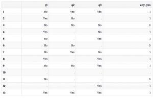
You should see that as long as a particular row has a value of Yes for at least one of q1, q2, or q3, it will have a value of 1 for any_yes. Notice that in rows 6 and 11, nonmissing values are all equal to No, so the resulting value of any_yes is 0. Also notice that the only case with a missing value for any_yes is row 10, which has missing values for all three of q1, q2, and q3.
What does this mean? If we go back to the ADHD example used at the start of this section, it implies that anyone whose mother, father, or biological sibling has been diagnosed with ADHD, is themselves considered to have a risk factor for ADHD. It does not assign “extra risk” if someone has two or more relatives that have been diagnosed.
8. Example: Using String Functions to Transform a Character Variable
When working with string variables — and especially when working with text data that’s been manually typed into the computer — your data values may have variation in capitalization. If you want to use this type of variable in an analysis, you’ll have to “standardize” the data values so that they all have the same patterns of capitalization, because SPSS considers each unique capitalization to be a different data value (even if the strings are otherwise identical).
A common string transformation is to convert a string to all uppercase or all lowercase characters. In SPSS, the functions UPCASE() and LOWER() will convert a string variable’s values to all uppercase characters or all lowercase characters, respectively.
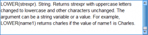
In the sample dataset, the variable Major is a string variable containing open-ended, write-in responses asking for the person’s college major. If you create a frequency table of this variable (Analyze > Descriptives > Frequencies), you’ll notice that there are many rows of the table, and that some of the rows of the table are identical except for differences in capitalization:
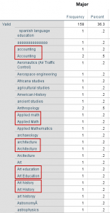
If we want to merge the otherwise-identical categories of “Art History” and “Art history”, we’ll need to transform this variable so that the characters are all uppercased or all lowercased.
Using the Compute Variables Dialog Window
- Click Transform > Compute Variables.
- In the Target Variable box, give the variable a new name, such as major_lowercase.
- Click Type & Label. Change the variable type to String, and set its length to 58. (This number comes from the length of the variable Major.)Click Continue to confirm and return to the Compute Variable window. Notice that in the Compute Variable window, the box where the formulas are entered is now labeled “String Expression” instead of “Numeric Expression”.
- In the String Expression box, enter the formula:
LOWER(Major) - When finished, click OK.
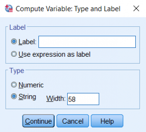 Click Continue to confirm and return to the Compute Variable window. Notice that in the Compute Variable window, the box where the formulas are entered is now labeled “String Expression” instead of “Numeric Expression”.
Using Syntax
STRING major_lowercase (A58).
COMPUTE major_lowercase = LOWER(Major).
EXECUTE.
Result
After executing the transformation and rerunning the frequency table on the transformed variable, we should see that the counts and frequencies of the previously duplicated categories are now combined:
![]()
While this variable is still not ready for analysis — for example, several duplicated categories exist because of misspellings or minor variations in wording — we have now completed the first step.
20 Sep 2022
28 Mar 2023
17 Sep 2022
20 Sep 2022
28 Mar 2023
20 Sep 2022