Testing for Significance for Simple Linear Regression

In a simple linear regression equation, the mean or expected value of y is a linear func­tion of x: E(y) = β₀ + β₁x. If the value of β₁ is zero, E(y) = β₀ + (0)x = b₀. In this case, the mean value of y does not depend on the value of x and hence we would conclude that x and y are not linearly related. Alternatively, if the value of β₁ is not equal to zero, we would conclude that the two variables are related. Thus, to test for a significant regression relationship, we must conduct a hypothesis test to determine whether the value of β₁ is zero. Two tests are commonly used. Both require an estimate of σ², the variance of e in the regression model.

1. Estimate of σ²

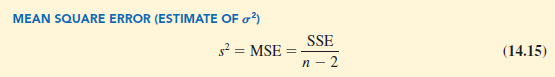
From the regression model and its assumptions we can conclude that σ², the variance of e, also represents the variance of the y values about the regression line. Recall that the deviations of the y values about the estimated regression line are called residuals. Thus, SSE, the sum of squared residuals, is a measure of the variability of the actual observations about the estimated regression line. The mean square error (MSE) provides the estimate of σ²; it is SSE divided by its degrees of freedom.

Every sum of squares has associated with it a number called its degrees of freedom. Statisticians have shown that SSE has n – 2 degrees of freedom because two parameters (β₀ and β₁) must be estimated to compute SSE. Thus, the mean square error is computed by dividing SSE by n – 2. MSE provides an unbiased estimator of σ². Because the value of MSE provides an estimate of a², the notation s² is also used.

In Section 14.3 we showed that for the Armand’s Pizza Parlors example, SSE = 1530; hence,

provides an unbiased estimate of σ².

To estimate a we take the square root of s². The resulting value, s, is referred to as the standard error of the estimate.

For the Armand’s Pizza Parlors example, s = VMSE = V191.25 = 13.829. In the fol­lowing discussion, we use the standard error of the estimate in the tests for a significant relationship between x and y.

2. t Test

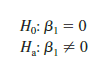
The simple linear regression model is y = β₀ + β1^x + ∈. If x and y are linearly related, we must have β₁ # 0. The purpose of the t test is to see whether we can conclude that β₁ # 0. We will use the sample data to test the following hypotheses about the para­meter β₁.

If H₀ is rejected, we will conclude that β₁ # 0 and that a statistically significant rela­tionship exists between the two variables. However, if H₀ cannot be rejected, we will have insufficient evidence to conclude that a significant relationship exists. The properties of the sampling distribution of b₁, the least squares estimator of β₁, provide the basis for the hypothesis test.

First, let us consider what would happen if we used a different random sample for the same regression study. For example, suppose that Armand’s Pizza Parlors used the sales records of a different sample of 10 restaurants. A regression analysis of this new sample might result in an estimated regression equation similar to our previous estimated regres­sion equation y = 60 + 5x. However, it is doubtful that we would obtain exactly the same equation (with an intercept of exactly 60 and a slope of exactly 5). Indeed, b₀ and b₁, the least squares estimators, are sample statistics with their own sampling distributions. The properties of the sampling distribution of b₁ follow.

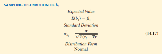
Note that the expected value of b₁ is equal to β₁, so b₁ is an unbiased estimator of β₁.

Because we do not know the value of s, we develop an estimate of σ_b, denoted σ_b1,, by estimating σ with s in equation (14.17). Thus, we obtain the following estimate of σ_b1..

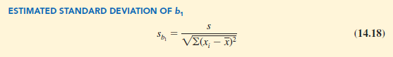
For Armand’s Pizza Parlors, s = 13.829. Hence, using Σ(x_i – X)² = 568 as shown in Table 14.2, we have

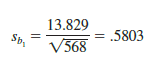
as the estimated standard deviation of b₁.

The t test for a significant relationship is based on the fact that the test statistic

follows a t distribution with n – 2 degrees of freedom. If the null hypothesis is true, then b₁ = 0 and t = b₁/s_b.

Let us conduct this test of significance for Armand’s Pizza Parlors at the a = .01 level of significance. The test statistic is

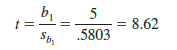
The t distribution table (Table 2 of Appendix D) shows that with n – 2 = 10 – 2 = 8 degrees of freedom, t = 3.355 provides an area of .005 in the upper tail. Thus, the area in the upper tail of the t distribution corresponding to the test statistic t = 8.62 must be less than .005. Because this test is a two-tailed test, we double this value to conclude that the p-value associated with t = 8.62 must be less than 2(.005) = .01. Statistical software shows the p-value = .000. Because the p-value is less than a = .01, we reject H₀ and conclude that β₁ is not equal to zero. This evidence is sufficient to conclude that a significant relationship exists between student population and quarterly sales. A summary of the t test for significance in simple linear regression follows.

3. Confidence Interval for β₁

The form of a confidence interval for b₁ is as follows:

The point estimator is b₁ and the margin of error is t_a/2s_b. The confidence coefficient associated with this interval is 1 – a, and t_a/2 is the t value providing an area of a/2 in the upper tail of a t distribution with n – 2 degrees of freedom. For example, suppose that we wanted to develop a 99% confidence interval estimate of b₁ for Armand’s Pizza Parlors. From Table 2 of Appendix B we find that the t value corresponding to a = .01 and n – 2 = 10 – 2 = 8 degrees of freedom is t.₀₀₅ = 3.355. Thus, the 99% confidence interval estimate of β₁ is

or 3.05 to 6.95.

In using the t test for significance, the hypotheses tested were

At the a = .01 level of significance, we can use the 99% confidence interval as an altern­ative for drawing the hypothesis testing conclusion for the Armand’s data. Because 0, the hypothesized value of β₁, is not included in the confidence interval (3.05 to 6.95), we can reject H₀ and conclude that a significant statistical relationship exists between the size of the student population and quarterly sales. In general, a confidence interval can be used to test any two-sided hypothesis about β₁. If the hypothesized value of β₁ is contained in the confidence interval, do not reject H₀. Otherwise, reject H₀.

4. F Test

An F test, based on the F probability distribution, can also be used to test for significance in regression. With only one independent variable, the F test will provide the same conclu­sion as the t test; that is, if the t test indicates β₁ # 0 and hence a significant relationship, the F test will also indicate a significant relationship. But with more than one independent variable, only the F test can be used to test for an overall significant relationship.

The logic behind the use of the F test for determining whether the regression relation­ship is statistically significant is based on the development of two independent estimates of σ². We explained how MSE provides an estimate of σ². If the null hypothesis H₀: β₁ = 0 is true, the sum of squares due to regression, SSR, divided by its degrees of freedom provides another independent estimate of σ². This estimate is called the mean square due to regression,or simply the mean square regression, and is denoted  MSR. In general,

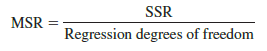
For the models we consider in this text, the regression degrees of freedom is always equal to the number of independent variables in the model:

Because we consider only regression models with one independent variable in this chapter, we have MSR = SSR/1 = SSR. Hence, for Armand’s Pizza Parlors, MSR = SSR = 14,200.

If the null hypothesis (H₀: β₁ = 0) is true, MSR and MSE are two independent estimates of σ² and the sampling distribution of MSR/MSE follows an F distribution with numer­ator degrees of freedom equal to one and denominator degrees of freedom equal to n — 2. Therefore, when b₁ = 0, the value of MSR/MSE should be close to one. However, if the null hypothesis is false (b₁ ^ 0), MSR will overestimate s² and the value of MSR/MSE will be inflated; thus, large values of MSR/MSE lead to the rejection of H₀ and the conclu­sion that the relationship between x and y is statistically significant.

Let us conduct the F test for the Armand’s Pizza Parlors example. The test statistic is

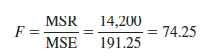
The F distribution table (Table 4 of Appendix B) shows that with one degree of freedom in the numerator and n — 2 = 10 — 2 = 8 degrees of freedom in the denominator, F = 11.26 provides an area of .01 in the upper tail. Thus, the area in the upper tail of the F distribution corresponding to the test statistic F = 74.25 must be less than .01. Thus, we conclude that the p-value must be less than .01. Statistical software shows the p-value = .000. Because the p-value is less than a = .01, we reject H₀ and conclude that a significant relationship exists between the size of the student population and quarterly sales. A summary of the F test for significance in simple linear regression follows.

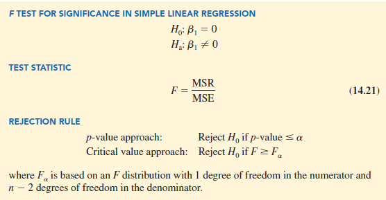
In Chapter 13 we covered analysis of variance (ANOVA) and showed how an ANOVA table could be used to provide a convenient summary of the computational aspects of analysis of variance. A similar ANOVA table can be used to summarize the results of the F test for significance in regression. Table 14.5 is the general form of the ANOVA table for simple linear regression. Table 14.6 is the ANOVA table with the F test computations performed for Armand’s Pizza Parlors. Regression, Error, and Total are the labels for the three sources of variation, with SSR, SSE, and SST appearing as the corresponding sum of squares in column 2. The degrees of freedom, 1 for SSR, n – 2 for SSE, and n – 1 for SST, are shown in column 3. Column 4 contains the values of MSR and MSE, column 5 contains the value of F = MSR/MSE, and column 6 contains the p-value corresponding to the F value in column 5. Almost all computer printouts of regression analysis include an ANOVA table summary of the F test for significance.

5. Some Cautions About the Interpretation of Significance Tests

Rejecting the null hypothesis H₀: β₁ = 0 and concluding that the relationship between x and y is significant does not enable us to conclude that a cause-and-effect relationship is present between x and y. Concluding a cause-and-effect relationship is warranted only if the analyst can provide some type of theoretical justification that the relationship is in fact causal. In the Armand’s Pizza Parlors example, we can conclude that there is a significant relationship between the size of the student population x and quarterly sales y; moreover, the estimated regression equation y = 60 + 5x provides the least squares estimate of the relationship. We cannot, however, conclude that changes in student population x cause changes in quarterly sales y just because we identified a statistically significant relation­ship. The appropriateness of such a cause-and-effect conclusion is left to supporting the­oretical justification and to good judgment on the part of the analyst. Armand’s managers felt that increases in the student population were a likely cause of increased quarterly sales. Thus, the result of the significance test enabled them to conclude that a cause-and-effect relationship was present.

In addition, just because we are able to reject H₀: β₁ = 0 and demonstrate statistical significance does not enable us to conclude that the relationship between x and y is linear.

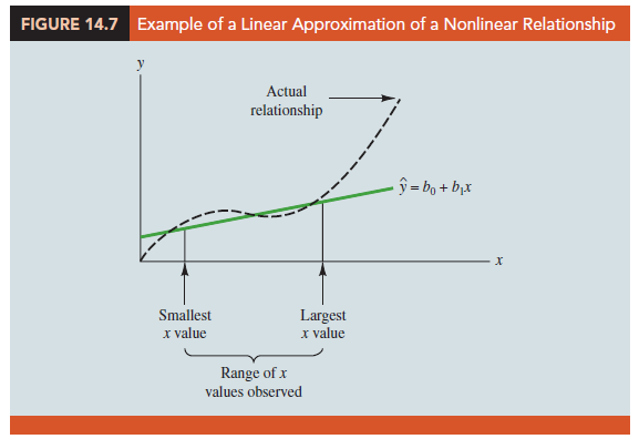
We can state only that x and y are related and that a linear relationship explains a signi­ficant portion of the variability in y over the range of values for x observed in the sample. Figure 14.7 illustrates this situation. The test for significance calls for the rejection of the null hypothesis H₀: β₁ = 0 and leads to the conclusion that x and y are significantly related, but the figure shows that the actual relationship between x and y is not linear. Although the linear approximation provided by y = b₀ + b₁x is good over the range of x values observed in the sample, it becomes poor for x values outside that range.

Given a significant relationship, we should feel confident in using the estimated regression equation for predictions corresponding to x values within the range of the x values observed in the sample. For Armand’s Pizza Parlors, this range corresponds to values of x between 2 and 26. Unless other reasons indicate that the model is valid beyond this range, predictions outside the range of the independent variable should be made with caution. For Armand’s Pizza Parlors, because the regression relationship has been found significant at the .01 level, we should feel confident using it to predict sales for restaurants where the associated student population is between 2000 and 26,000.

Source:  Anderson David R., Sweeney Dennis J., Williams Thomas A. (2019), Statistics for Business & Economics, Cengage Learning; 14th edition.