Using the Estimated Simple Linear Regression Equation for Estimation and Prediction

When using the simple linear regression model, we are making an assumption about the relationship between x and y. We then use the least squares method to obtain the estimated simple linear regression equation. If a significant relationship exists between x and y and the coefficient of determination shows that the fit is good, the estimated regression equation should be useful for estimation and prediction.

For the Armand’s Pizza Parlors example, the estimated regression equation is y = 60 + 5x.

At the end of Section 14.1, we stated that y can be used as a point estimator of E(y), the mean or expected value of y for a given value of x, and as a predictor of an individual value of y. For ex­ample, suppose Armand’s managers want to estimate the mean quarterly sales for all restaurants located near college campuses with 10,000 students. Using the estimated regression equation y = 60 + 5x, we see that for x = 10 (10,000 students), y = 60 + 5(10) = 110. Thus, a point estimate of the mean quarterly sales for all restaurant locations near campuses with 10,000 students is $110,000. In this case we are using y as the point estimator of the mean value of y when x = 10.

We can also use the estimated regression equation to predict an individual value of y for a given value of x. For example, to predict quarterly sales for a new restaurant Armand’s is considering building near Talbot College, a campus with 10,000 students, we would compute y = 60 + 5(10) = 110. Hence, we would predict quarterly sales of $110,000 for such a new restaurant. In this case, we are using y as the predictor of y for a new observation when x = 10.

When we are using the estimated regression equation to estimate the mean value of y or to predict an individual value of y, it is clear that the estimate or prediction depends on the given value of x. For this reason, as we discuss in more depth the issues concerning estimation and prediction, the following notation will help clarify matters.

x* = the given value of the independent variable x

y* = the random variable denoting the possible values of the dependent variable y when x = x*

E(y*) = the mean or expected value of the dependent variable y when x = x*

y* = b₀ + b₁x* = the point estimator of E(y*) and the predictor of an individual value of y* when x = x*

To illustrate the use of this notation, suppose we want to estimate the mean value of quarterly sales for all Armand’s restaurants located near a campus with 10,000 students. For this case, x* = 10 and E(y*) denotes the unknown mean value of quarterly sales for all restaurants where x* = 10. Thus, the point estimate of E(y*) is provided by y* = 60 + 5(10) = 110, or $110,000. But, using this notation, y* = 110 is also the predictor of quarterly sales for the new restaurant located near Talbot College, a school with 10,000 students.

1. Interval Estimation

Point estimators and predictors do not provide any information about the precision associated with the estimate and/or prediction. For that we must develop confidence intervals and prediction intervals. A confidence interval is an interval estimate of the mean value of y for a given value of x. A prediction interval is used whenever we want to predict an individual value of y for a new observation corresponding to a given value of x. Although the predictor of y for a given value of x is the same as the point estimator of the mean value of y for a given value of x, the interval estimates we obtain for the two cases are different. As we will show, the margin of error is larger for a prediction interval. We begin by showing how to develop an interval estimate of the mean value of y.

2. Confidence Interval for the Mean Value of y

In general, we cannot expect y* to equal E(y*) exactly. If we want to make an inference about how close y* is to the true mean value E(y*), we will have to estimate the variance of y*. The formula for estimating the variance of y*, denoted by s2y*, is

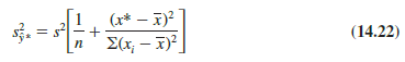
The estimate of the standard deviation of y* is given by the square root of equation (14.22).

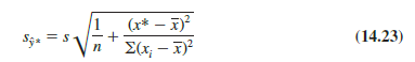
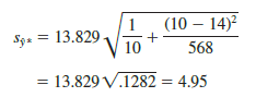
The computational results for Armand’s Pizza Parlors in Section 14.5 provided s = 13.829. With x* = 10, X = 14, and ∑(x_i – X)² = 568, we can use equation (14.23) to obtain

The general expression for a confidence interval follows.

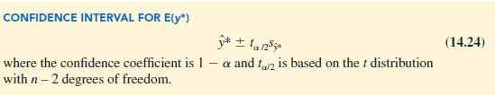
Using expression (14.24) to develop a 95% confidence interval of the mean quarterly sales for all Armand’s restaurants located near campuses with 10,000 students, we need the value of t for a/2 = .025 and n – 2 = 10 – 2 = 8 degrees of freedom. Using Table 2 of Appendix B, we have t.₀₂₅ = 2.306. Thus, with y* = 110 and a margin of error of t_a/2Sy* = 2.306(4.95) = 11.415, the 95% confidence interval estimate is

In dollars, the 95% confidence interval for the mean quarterly sales of all restaurants near cam­puses with 10,000 students is $110,000 ± $11,415. Therefore, the 95% confidence interval for the mean quarterly sales when the student population is 10,000 is $98,585 to $121,415.

Note that the estimated standard deviation of y* given by equation (14.23) is smallest when x* – x = 0. In this case the estimated standard deviation of y* becomes

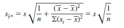
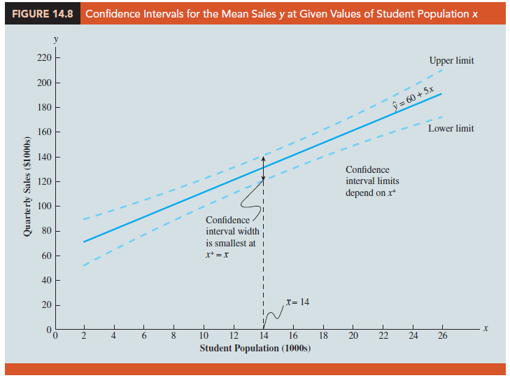
This result implies that we can make the best or most precise estimate of the mean value of y whenever x* = x. In fact, the further x* is from x, the larger x* – x becomes. As a result, the confidence interval for the mean value of y will become wider as x* deviates more from x. This pattern is shown graphically in Figure 14.8.

3. Prediction Interval for an Individual Value of y

Instead of estimating the mean value of quarterly sales for all Armand’s restaurants located near campuses with 10,000 students, suppose we want to predict quarterly sales for a new res­taurant Armand’s is considering building near Talbot College, a campus with 10,000 students. As noted previously, the predictor of y*, the value of y corresponding to the given x*, is y* = b₀ + ^b1^x*. For the new restaurant located near Talbot College, x* = 10 and the prediction of quarterly sales is y* = 60 + 5(10) = 110, or $110,000. Note that the prediction of quarterly sales for the new Armand’s restaurant near Talbot College is the same as the point estimate of the mean sales for all Armand’s restaurants located near campuses with 10,000 students.

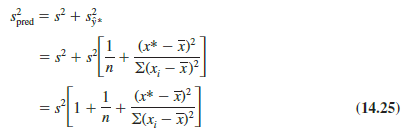
To develop a prediction interval, let us first determine the variance associated with using y* as a predictor of y when x = x*. This variance is made up of the sum of the following two components.

1. The variance of the y* values about the mean E(y*), an estimate of which is given by s²
2. The variance associated with using y* to estimate E(y*), an estimate of which is given by s²y*

The formula for estimating the variance corresponding to the prediction of the value of y when x = x*, denoted s²pred , is

Hence, an estimate of the standard deviation corresponding to the prediction of the value of y* is

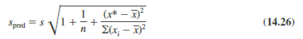
For Armand’s Pizza Parlors, the estimated standard deviation corresponding to the pre­diction of quarterly sales for a new restaurant located near Talbot College, a campus with 10,000 students, is computed as follows.

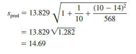
The general expression for a prediction interval follows.

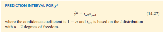
The 95% prediction interval for quarterly sales for the new Armand’s restaurant located near Talbot College can be found using t_a/2 = t.₀₂₅ = 2.306 and s_pred = 14.69. Thus, with y* = 110 and a margin of error of t_.025s_pred = 2.306(14.69) = 33.875, the 95% prediction interval is

110 ± 33.875

In dollars, this prediction interval is $110,000 ± $33,875 or $76,125 to $143,875. Note that the prediction interval for the new restaurant located near Talbot College, a campus with 10,000 students, is wider than the confidence interval for the mean quarterly sales of all restaurants located near campuses with 10,000 students. The difference reflects the fact that we are able to estimate the mean value of y more precisely than we can predict an individual value of y.

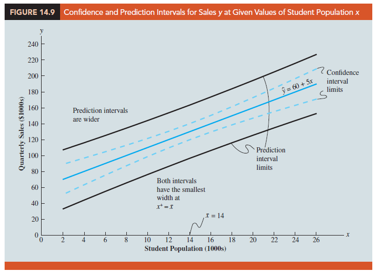
Confidence intervals and prediction intervals are both more precise when the value of the independent variable x* is closer to x. The general shapes of confidence intervals and the wider prediction intervals are shown together in Figure 14.9.

Source:  Anderson David R., Sweeney Dennis J., Williams Thomas A. (2019), Statistics for Business & Economics, Cengage Learning; 14th edition.