Inferences About a Population Variance

The sample variance

is the point estimator of the population variance s². In using the sample variance as a basis for making inferences about a population variance, the sampling distribution of the quan­tity (n – 1)s¹/s² is helpful. This sampling distribution is described as follows.

Figure 11.1 shows some possible forms of the sampling distribution of (n − 1)s2/σ2.

Because the sampling distribution of (n – 1)s ²/σ² is known to have a chi-square distribution whenever a simple random sample of size n is selected from a normal pop­ulation, we can use the chi-square distribution to develop interval estimates and conduct hypothesis tests about a population variance.

1. Interval Estimation

To show how the chi-square distribution can be used to develop a confidence interval estimate of a population variance σ², suppose that we are interested in estimating the population variance for the production filling process mentioned at the beginning of this chapter. A sample of 20 containers is taken, and the sample variance for the filling quan­tities is found to be s² = .0025. However, we know we cannot expect the variance of a sample of 20 containers to provide the exact value of the variance for the population of containers filled by the production process. Hence, our interest will be in developing an interval estimate for the population variance.

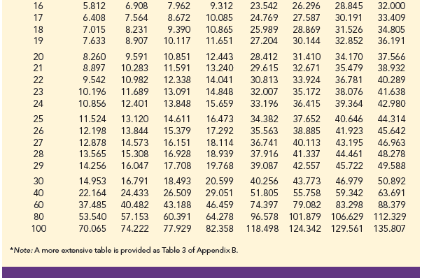
We will use the notation x2a to denote the value for the chi-square distribution that provides an area or probability of a to the right of the x2a value. For example, in Figure 11.2 the chi-square distribution with 19 degrees of freedom is shown with X₀₂₅ = 32.852 indicating that 2.5% of the chi-square values are to the right of 32.852, and X²975 = 8.907 indicating that 97.5% of the chi-square values are to the right of 8.907. Tables of areas or probabilities are readily available for the chi-square distribution. Refer to Table 11.1 and verify that these chi-square values with 19 degrees of freedom (19th row of the table) are correct. Table 3 of Appendix B provides a more extensive table of chi-square values.

From the graph in Figure 11.2 we see that .95, or 95%, of the chi-square values are between x²₉₇₅ and x²₀₂₅. That is, there is a .95 probability of obtaining a X² value such that

We stated in expression (11.2) that (n – 1)s²/σ² follows a chi-square distribution; therefore we can substitute (n – 1)s²/σ² for x² and write

In effect, expression (11.3) provides an interval estimate in that .95, or 95%, of all possible values for (n – 1)s²/σ² will be in the interval x²₉₇₅ to x²₀₂₅. We now need to do some algebraic manipulations with expression (11.3) to develop an interval estimate for the population variance σ². Working with the leftmost inequality in expression (11.3), we have

Performing similar algebraic manipulations with the rightmost inequality in expres­sion (11.3) gives

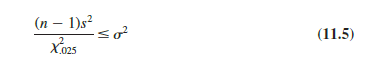
The results of expressions (11.4) and (11.5) can be combined to provide

Because expression (11.3) is true for 95% of the (n – 1) s²/σ² values, expression (11.6) provides a 95% confidence interval estimate for the population variance s².

Let us return to the problem of providing an interval estimate for the population vari­ance of filling quantities. Recall that the sample of 20 containers provided a sample vari­ance of s² = .0025. With a sample size of 20, we have 19 degrees of freedom. As shown in Figure 11.2, we have already determined that x²₉₇₅ = 8.907 and x²₀₂₅ = 32.852. Using these values in expression (11.6) provides the following interval estimate for the population variance.

Taking the square root of these values provides the following 95% confidence interval for the population standard deviation.

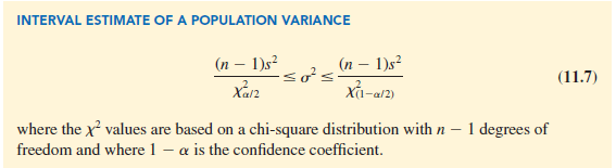
Thus, we illustrated the process of using the chi-square distribution to establish interval estimates of a population variance and a population standard deviation. Note specifically that because x²₉₇₅ and x²₀₂₅ were used, the interval estimate has a .95 confidence coefficient. Extending expression (11.6) to the general case of any confidence coefficient, we have the following interval estimate of a population variance.

2. Hypothesis Testing

Using s0 to denote the hypothesized value for the population variance, the three forms for a hypothesis test about a population variance are as follows:

These three forms are similar to the three forms used to conduct one-tailed and two-tailed hypothesis tests about population means and proportions.

The procedure for conducting a hypothesis test about a population variance uses the hypothesized value for the population variance sO and the sample variance s² to compute the value of a X² test statistic. Assuming that the population has a normal distribution, the test statistic is as follows:

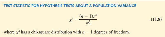
After computing the value of the x² test statistic, either the p-value approach or the critical value approach, may be used to determine whether the null hypothesis can be rejected.

Let us consider the following example. The St. Louis Metro Bus Company wants to promote an image of reliability by encouraging its drivers to maintain consistent schedules. As a standard policy, the company would like arrival times at bus stops to have low vari­ability. In terms of the variance of arrival times, the company standard specifies an arrival time variance of 4 or less when arrival times are measured in minutes. The following hypo­thesis test is formulated to help the company determine whether the arrival time population variance is excessive.

In tentatively assuming H₀ is true, we are assuming that the population variance of arrival times is within the company guideline. We reject H₀ if the sample evidence indicates that the population variance exceeds the guideline. In this case, follow-up steps should be taken to reduce the population variance. We conduct the hypothesis test using a level of significance of a = .05.

Suppose that a random sample of 24 bus arrivals taken at a downtown intersection provides a sample variance of s² = 4.9. Assuming that the population distribution of arrival times is approximately normal, the value of the test statistic is as follows.

The chi-square distribution with n − 1 = 24 − 1 = 23 degrees of freedom is shown in Figure 11.3. Because this is an upper tail test, the area under the curve to the right of the test statistic x2 = 28.18 is the p-value for the test.

Like the t distribution table, the chi-square distribution table does not contain sufficient detail to enable us to determine the p-value exactly. However, we can use the chi-square distribution table to obtain a range for the p-value. For example, using Table 11.1, we find the following information for a chi-square distribution with 23 degrees of freedom.

Because x2 = 28.18 is less than 32.007, the area in upper tail (the p-value) is greater than .10. With the p-value . a = .05, we cannot reject the null hypothesis. The sample does not support the conclusion that the population variance of the arrival times is
excessive.

Because of the difficulty of determining the exact p-value directly from the chi-square distribution table, statistical software is helpful. Appendix F, at the back of the book, describes how to compute p-values using JMP or Excel. In the appendix, we show that the exact p-value corresponding to x2 = 28.18 is .2091.

As with other hypothesis testing procedures, the critical value approach can also be used to draw the hypothesis testing conclusion. With a = .05, x2 .05 provides the critical value for the upper tail hypothesis test. Using Table 11.1 and 23 degrees of freedom, X₀₅ = 35.172. Thus, the rejection rule for the bus arrival time example is as follows:

Because the value of the test statistic is X² = 28.18, we cannot reject the null hypothesis.

In practice, upper tail tests as presented here are the most frequently encountered tests about a population variance. In situations involving arrival times, production times, filling weights, part dimensions, and so on, low variances are desirable, whereas large variances are unacceptable. With a statement about the maximum allowable population variance, we can test the null hypothesis that the population variance is less than or equal to the max­imum allowable value against the alternative hypothesis that the population variance is greater than the maximum allowable value. With this test structure, corrective action will be taken whenever rejection of the null hypothesis indicates the presence of an excessive population variance.

As we saw with population means and proportions, other forms of hypothesis tests can be developed. Let us demonstrate a two-tailed test about a population variance by consider­ing a situation faced by a bureau of motor vehicles. Historically, the variance in test scores for individuals applying for driver’s licenses has been s² = 100. A new examination with new test questions has been developed. Administrators of the bureau of motor vehicles would like the variance in the test scores for the new examination to remain at the historical level. To evaluate the variance in the new examination test scores, the following two-tailed hypothesis test has been proposed.

Rejection of H₀ will indicate that a change in the variance has occurred and suggest that some questions in the new examination may need revision to make the variance of the new test scores similar to the variance of the old test scores. A sample of 30 applicants for driver’s licenses will be given the new version of the examination. We will use a level of significance a = .05 to conduct the hypothesis test.

The sample of 30 examination scores provided a sample variance s² = 162. The value of the chi-square test statistic is as follows:

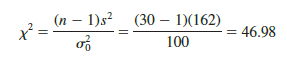
Now, let us compute the p-value. Using Table 11.1 and n – 1 = 30 – 1 = 29 degrees of freedom, we find the following.

Thus, the value of the test statistic x² = 46.98 provides an area between .025 and .01 in the upper tail of the chi-square distribution. Doubling these values shows that the two-tailed p-value is between .05 and .02. Statistical software can be used to show the exact p-value = .0374. With p-value < a = .05, we reject H₀ and conclude that the new examination test scores have a population variance different from the historical variance of σ² = 100. A sum­mary of the hypothesis testing procedures for a population variance is shown in Table 11.2.

Source:  Anderson David R., Sweeney Dennis J., Williams Thomas A. (2019), Statistics for Business & Economics, Cengage Learning; 14th edition.