Testing the Equality of Population Proportions for Three or More Populations

In this section, we show how the chi-square (^²) test statistic can be used to make statist­ical inferences about the equality of population proportions for three or more populations. Using the notation

the hypotheses for the equality of population proportions for k > 3 populations are as follows:

If the sample data and the chi-square test computations indicate H₀ cannot be rejected, we cannot detect a difference among the k population proportions. However, if the sample data and the chi-square test computations indicate H₀ can be rejected, we have the stat­istical evidence to conclude that not all k population proportions are equal; that is, one or more population proportions differ from the other population proportions. Further analyses can be done to conclude which population proportion or proportions are signi­ficantly different from others. Let us demonstrate this chi-square test by considering an application.

Organizations such as J.D. Power and Associates use the proportion of owners likely to repurchase a particular automobile as an indication of customer loyalty for the automobile. An automobile with a greater proportion of owners likely to repur­chase is concluded to have greater customer loyalty. Suppose that in a particular study we want to compare the customer loyalty for three automobiles: Chevrolet Impala, Ford Fusion, and Honda Accord. The current owners of each of the three automobiles form the three populations for the study. The three population proportions of interest are as follows:

p₁ = proportion likely to repurchase an Impala for the population of Chevrolet Impala owners

p₂ = proportion likely to repurchase a Fusion for the population of Ford Fusion owners

p₃ = proportion likely to repurchase an Accord for the population of Honda Accord owners

The hypotheses are stated as follows:

To conduct this hypothesis test we begin by taking a sample of owners from each of the three populations. Thus we will have a sample of Chevrolet Impala owners, a sample of Ford Fusion owners, and a sample of Honda Accord owners. Each sample provides categorical data indicating whether the respondents are likely or not likely to repurchase the automobile. The data for samples of 125 Chevrolet Impala owners, 200 Ford Fusion owners, and 175 Honda Accord owners are summarized in the tabular format shown in Table 12.1. This table has two rows for the responses Yes and No and three columns, one corresponding to each of the pop­ulations. The observed frequencies are summarized in the six cells of the table corresponding to each combination of the likely to repurchase responses and the three populations.

Using Table 12.1, we see that 69 of the 125 Chevrolet Impala owners indicated that they were likely to repurchase a Chevrolet Impala. One hundred and twenty of the 200 Ford Fusion owners and 123 of the 175 Honda Accord owners indicated that they were likely to repurchase their current automobile. Also, across all three samples, 312 of the 500 owners in the study indicated that they were likely to repurchase their current auto­mobile. The question now is how do we analyze the data in Table 12.1 to determine if the hypothesis H₀: p₁ = p₂ = p₃ should be rejected?

The data in Table 12.1 are the observed frequencies for each of the six cells that repres­ent the six combinations of the likely to repurchase response and the owner population. If we can determine the expected frequencies under the assumption H₀ is true, we can use the chi-square test statistic to determine whether there is a significant difference between the observed and expected frequencies. If a significant difference exists between the observed and expected frequencies, the hypothesis H₀ can be rejected and there is evidence that not all the population proportions are equal.

Expected frequencies for the six cells of the table are based on the following rationale. First, we assume that the null hypothesis of equal population proportions is true. Then we note that in the entire sample of 500 owners, a total of 312 owners indicated that they were likely to repurchase their current automobile. Thus, 312/500 = .624 is the overall sample proportion of owners indicating they are likely to repurchase their current automobile. If H₀: p₁ = p₂ = p₃ is true, .624 would be the best estimate of the proportion responding likely to repurchase for each of the automobile owner populations. So if the assumption of H₀ is true, we would expect .624 of the 125 Chevrolet Impala owners, or .624(125) = 78 owners to indicate they are likely to repurchase the Impala. Using the .624 overall sample proportion, we would expect .624(200) = 124.8 of the 200 Ford Fusion owners and .624(175) = 109.2 of the Honda Accord owners to respond that they are likely to repurchase their respective model of automobile.

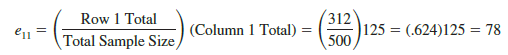
Let us generalize the approach to computing expected frequencies by letting e_tj denote the expected frequency for the cell in row i and column j of the table. With this notation, now reconsider the expected frequency calculation for the response of likely to repurchase Yes (row 1) for Chevrolet Impala owners (column 1), that is, the expected frequency e₁₁.

Note that 312 is the total number of Yes responses (row 1 total), 175 is the total sample size for Chevrolet Impala owners (column 1 total), and 500 is the total sample size. Following the logic in the preceding paragraph, we can show

Starting with the first part of the above expression, we can write

Using equation (12.1), we see that the expected frequency of Yes responses (row 1) for Honda Accord owners (column 3) would be e13 = (Row 1 Total)(Column 3 Total)/(Total Sample Size) = (312)(175)/500 = 109.2. Use equation (12.1) to verify the other expected frequencies are as shown in Table 12.2.

The test procedure for comparing the observed frequencies of Table 12.1 with the expected frequencies of Table 12.2 involves the computation of the following chi-square statistic:

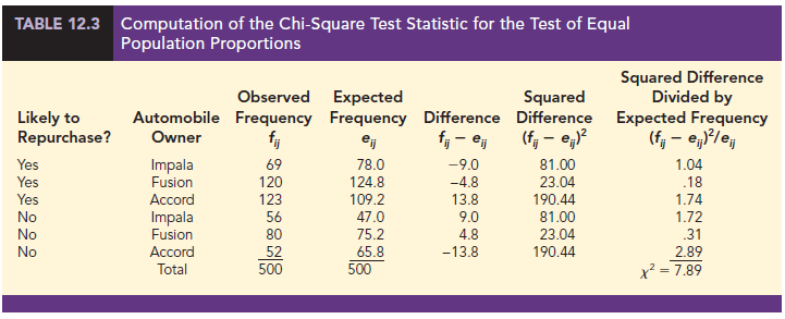
Reviewing the expected frequencies in Table 12.2, we see that the expected frequency is at least five for each cell in the table. We therefore proceed with the computation of the chi-square test statistic. The calculations necessary to compute the value of the test statistic are shown in Table 12.3. In this case, we see that the value of the test statistic is x2 = 7.89.

In order to understand whether or not x² = 7.89 leads us to reject H₀: p₁ = p₂ = p₃, you will need to understand and refer to values of the chi-square distribution. Table 12.4 shows the general shape of the chi-square distribution, but note that the shape of a specific chi-square distribution depends upon the number of degrees of freedom. The table shows the upper tail areas of .10, .05, .025, .01, and .005 for chi-square distributions with up to 15 degrees of freedom. This version of the chi-square table will enable you to conduct the hypothesis tests presented in this chapter.

Since the expected frequencies shown in Table 12.2 are based on the assumption that H₀: p₁ = p₂ = p₃ is true, observed frequencies,fj, that are in agreement with expected frequencies, e_tj, provide small values of f – e_tj)² in equation (12.2). If this is the case, the value of the chi-square test statistic will be relatively small and H₀ cannot be rejected. On the other hand, if the differences between the observed and expected frequencies are large, values of (fj – ej)¹ and the computed value of the test statistic will be large. In this case, the null hypothesis of equal population proportions can be rejected. Thus a chi-square test for equal population proportions will always be an upper tail test with rejection of H₀ occurring when the test statistic is in the upper tail of the chi-square distribution.

We can use the upper tail area of the appropriate chi-square distribution and the p-value approach to determine whether the null hypothesis can be rejected. In the auto­mobile brand loyalty study, the three owner populations indicate that the appropriate chi-square distribution has k – 1 = 3 – 1 = 2 degrees of freedom. Using row two of the chi-square distribution table, we have the following:

We see the upper tail area at x² = 7.89 is between .025 and .01. Thus, the corresponding upper tail area or p-value must be between .025 and .01. With p-value < .05, we reject H₀ and conclude that the three population proportions are not all equal and thus there is a difference in brand loyalties among the Chevrolet Impala, Ford Fusion, and Honda Accord owners. JMP or Excel procedures provided in Appendix F can be used to show X² = 7.89 with 2 degrees of freedom yields a p-value = .0193.

Instead of using the p-value, we could use the critical value approach to draw the same conclusion. With a = .05 and 2 degrees of freedom, the critical value for the chi-square test statistic is x² = 5.991. The upper tail rejection region becomes

With 7.89 > 5.991, we reject H₀. Thus, the p-value approach and the critical value approach provide the same hypothesis-testing conclusion.

Let us summarize the general steps that can be used to conduct a chi-square test for the equality of the population proportions for three or more populations.

1. A Multiple Comparison Procedure

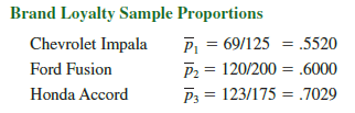
We have used a chi-square test to conclude that the population proportions for the three populations of automobile owners are not all equal. Thus, some differences among the population proportions exist and the study indicates that customer loyalties are not all the same for the Chevrolet Impala, Ford Fusion, and Honda Accord owners. To identify where the differences between population proportions exist, we can begin by computing the three sample proportions as follows:

Since the chi-square test indicated that not all population proportions are equal, it is reasonable for us to proceed by attempting to determine where differences among the population proportions exist. For this we will rely on a multiple comparison procedure that can be used to conduct statistical tests between all pairs of population proportions.

In the following, we discuss a multiple comparison procedure known as the Marascuilo procedure. This is a relatively straightforward procedure for making pairwise comparisons of all pairs of population proportions. We will demonstrate the computations required by this multiple comparison test procedure for the automobile customer loyalty study.

We begin by computing the absolute value of the pairwise difference between sample proportions for each pair of populations in the study. In the three-population automobile brand loyalty study we compare populations 1 and 2, populations 1 and 3, and then popula­tions 2 and 3 using the sample proportions as follows:

In a second step, we select a level of significance and compute the corresponding critical value for each pairwise comparison using the following expression.

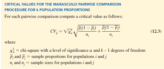
Using the chi-square distribution in Table 12.4, k – 1 = 3 – 1 = 2 degrees of free­dom, and a .05 level of significance, we have x²₀₅ = 5.991. Now using the sample propor­tions p₁ = .5520, p₂ = .6000, and p₃ = .7029, the critical values for the three pairwise comparison tests are as follows:

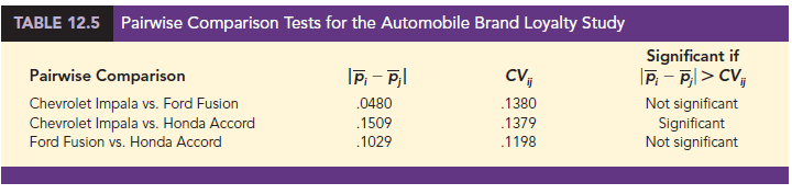
If the absolute value of any pairwise sample proportion difference | p_i – pj \ exceeds its corresponding critical value, CV_ij, the pairwise difference is significant at the .05 level of significance and we can conclude that the two corresponding population proportions are different. The final step of the pairwise comparison procedure is summarized in Table 12.5.

The conclusion from the pairwise comparison procedure is that the only significant difference in customer loyalty occurs between the Chevrolet Impala and the Honda Accord. Our sample results indicate that the Honda Accord had a greater population proportion of owners who say they are likely to repurchase the Honda Accord. Thus, we can conclude that the Honda Accord (p₃ = .7029) has a greater customer loyalty than the Chevrolet Impala (p₁ = .5520).

The results of the study are inconclusive as to the comparative loyalty of the Ford Fusion. While the Ford Fusion did not show significantly different results when compared to the Chevrolet Impala or Honda Accord, a larger sample may have revealed a significant differ­ence between Ford Fusion and the other two automobiles in terms of customer loyalty. It is not uncommon for a multiple comparison procedure to show significance for some pairwise comparisons and yet not show significance for other pairwise comparisons in the study.

Source:  Anderson David R., Sweeney Dennis J., Williams Thomas A. (2019), Statistics for Business & Economics, Cengage Learning; 14th edition.