Population Proportion

In the introduction to this chapter we said that the general form of an interval estimate of a population proportion p is

The sampling distribution of p plays a key role in computing the margin of error for this interval estimate.

In Chapter 7 we said that the sampling distribution of p can be approximated by a nor­mal distribution whenever np ≥ 5 and n(1 – p) ≥ 5. Figure 8.8 shows the normal approxi­mation of the sampling distribution of p. The mean of the sampling distribution of p is the population proportion p, and the standard error of p is

Because the sampling distribution of p is normally distributed, if we choose z_a/2σp as the margin of error in an interval estimate of a population proportion, we know that 100(1 – a)% of the intervals generated will contain the true population proportion. But sp cannot be used directly in the computation of the margin of error because p will not be known; p is what we are trying to estimate. So p is substituted for p and the margin of error for an interval estimate of a population proportion is given by

With this margin of error, the general expression for an interval estimate of a population proportion is as follows.

The following example illustrates the computation of the margin of error and interval estimate for a population proportion. A national survey of 900 women golfers was conduc­ted to learn how women golfers view their treatment at golf courses in the United States. The survey found that 396 of the women golfers were satisfied with the availability of tee times. Thus, the point estimate of the proportion of the population of women golfers who are satisfied with the availability of tee times is 396/900 = .44. Using expression (8.6) and a 95% confidence level,

Thus, the margin of error is .0324 and the 95% confidence interval estimate of the popula­tion proportion is .4076 to .4724. Using percentages, the survey results enable us to state with 95% confidence that between 40.76% and 47.24% of all women golfers are satisfied with the availability of tee times.

1. Determining the Sample Size

Let us consider the question of how large the sample size should be to obtain an estimate of a population proportion at a specified level of precision. The rationale for the sample size determination in developing interval estimates of – is similar to the rationale used in Section 8.3 to determine the sample size for estimating a population mean.

Previously in this section we said that the margin of error associated with an interval estimate of a population proportion is  The margin of error is based on the value of z_a2, the sample proportion -, and the sample size n. Larger sample sizes provide a smaller margin of error and better precision.

Let E denote the desired margin of error.

Solving this equation for n provides a formula for the sample size that will provide a mar­gin of error of size E.

Note, however, that we cannot use this formula to compute the sample size that will provide the desired margin of error because — will not be known until after we select the sample. What we need, then, is a planning value for – that can be used to make the compu­tation. Using -* to denote the planning value for -, the following formula can be used to compute the sample size that will provide a margin of error of size E.

In practice, the planning value p* can be chosen by one of the following procedures.

1. Use the sample proportion from a previous sample of the same or similar units.
2. Use a pilot study to select a preliminary sample. The sample proportion from this sample can be used as the planning value, p*.
3. Use judgment or a “best guess” for the value of p*.
4. If none of the preceding alternatives applies, use a planning value ofp* = .50.

Let us return to the survey of women golfers and assume that the company is interested in conducting a new survey to estimate the current proportion of the population of women golfers who are satisfied with the availability of tee times. How large should the sample be if the survey director wants to estimate the population proportion with a margin of error of .025 at 95% confidence? With E = .025 and z_a/2 = 1.96, we need a planning value p* to answer the sample size question. Using the previous survey result of p = .44 as the planning value p*, equation (8.7) shows that

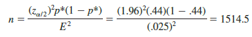
Thus, the sample size must be at least 1514.5 women golfers to satisfy the margin of error requirement. Rounding up to the next integer value indicates that a sample of 1515 women golfers is recommended to satisfy the margin of error requirement.

The fourth alternative suggested for selecting a planning value p* is to use p* = .50. This value of p* is frequently used when no other information is available. To understand why, note that the numerator of equation (8.7) shows that the sample size is proportional to the quantity p*(1 – p*). A larger value for the quantity p*(1 – p*) will result in a larger sample size. Table 8.5 gives some possible values of p*(1 – p*). Note that the largest value of p*(1 – p*) occurs when p* = .50. Thus, in case of any uncertainty about an appropriate planning value, we know that p* = .50 will provide the largest sample size recommend­ation. In effect, we play it safe by recommending the largest necessary sample size. If the sample proportion turns out to be different from the .50 planning value, the margin of error will be smaller than anticipated. Thus, in using p* = .50, we guarantee that the sample size will be sufficient to obtain the desired margin of error.

In the survey of women golfers example, a planning value of p* = .50 would have provided the sample size

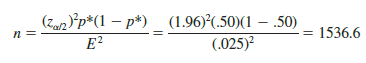
Thus, a slightly larger sample size of 1537 women golfers would be recommended.

Source:  Anderson David R., Sweeney Dennis J., Williams Thomas A. (2019), Statistics for Business & Economics, Cengage Learning; 14th edition.