In many regression applications, the dependent variable may only assume two discrete values. For instance, a bank might want to develop an estimated regression equation for predicting whether a person will be approved for a credit card. The dependent variable can be coded as y = 1 if the bank approves the request for a credit card and y = 0 if the bank rejects the request for a credit card. Using logistic regression we can estimate the probability that the bank will approve the request for a credit card given a particular set of values for the chosen independent variables.
Let us consider an application of logistic regression involving a direct mail promotion being used by Simmons Stores. Simmons owns and operates a national chain of women’s apparel stores. Five thousand copies of an expensive four-color sales catalog have been printed, and each catalog includes a coupon that provides a $50 discount on purchases of $200 or more. The catalogs are expensive and Simmons would like to send them to only those customers who have a high probability of using the coupon.
Management believes that annual spending at Simmons Stores and whether a customer has a Simmons credit card are two variables that might be helpful in predicting whether a customer who receives the catalog will use the coupon. Simmons conducted a pilot study using a random sample of 50 Simmons credit card customers and 50 other customers who do not have a Simmons credit card. Simmons sent the catalog to each of the 100 customers selected. At the end of a test period, Simmons noted whether each customer had used her or his coupon. The sample data for the first 10 catalog recipients are shown in Table 15.11.
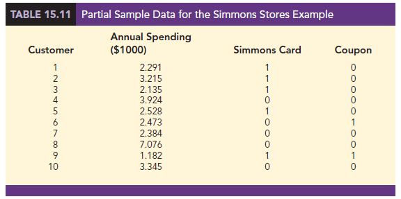
The amount each customer spent last year at Simmons is shown in thousands of dollars and the credit card information has been coded as 1 if the customer has a Simmons credit card and 0 if not. In the Coupon column, a 1 is recorded if the sampled customer used the coupon and 0 if not.
We might think of building a multiple regression model using the data in Table 15.11 to help Simmons estimate whether a catalog recipient will use the coupon. We would use Annual Spending ($1000) and Simmons Card as independent variables and Coupon as the dependent variable. Because the dependent variable may only assume the values of 0 or 1, however, the ordinary multiple regression model is not applicable. This example shows the type of situation for which logistic regression was developed. Let us see how logistic regression can be used to help Simmons estimate which type of customer is most likely to take advantage of their promotion.
1. Logistic Regression Equation
In many ways logistic regression is like ordinary regression. It requires a dependent variable, y, and one or more independent variables. In multiple regression analysis, the mean or expected value of y is referred to as the multiple regression equation.
![]()
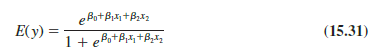
In logistic regression, statistical theory as well as practice has shown that the relationship between E(y) and x1, x2,…, xp is better described by the following nonlinear equation.

If the two values of the dependent variable y are coded as 0 or 1, the value of E(y) in equation (15.27) provides the probability that y = 1 given a particular set of values for the independent variables x1, x2, . . . , xp. Because of the interpretation of E(y) as a probability, the logistic regression equation is often written as follows:

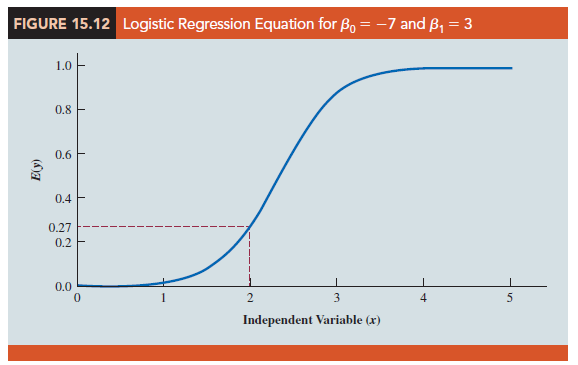
To provide a better understanding of the characteristics of the logistic regression equation, suppose the model involves only one independent variable x and the values of the model parameters are β0 = -7 and β1 = 3. The logistic regression equation corresponding to these parameter values is
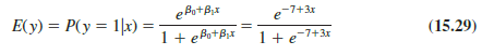 Figure 15.12 shows a graph of equation (15.29). Note that the graph is S-shaped. The value of E(y) ranges from 0 to 1. For example, when x = 2, E(y) is approximately .27. Also note that the value of E(y) gradually approaches 1 as the value of x becomes larger and the value of E(y) approaches 0 as the value of x becomes smaller. For example, when x = 2, E(y) = .269. Note also that the values of E(y), representing probability, increase fairly rapidly as x increases from 2 to 3. The fact that the values of E(y) range from 0 to 1 and that the curve is S-shaped makes equation (15.29) ideally suited to model the probability the dependent variable is equal to 1.
2. Estimating the Logistic Regression Equation
In simple linear and multiple regression the least squares method is used to compute b0, b1, . . . , bp as estimates of the model parameters (β0, β1 • • • , βp). The nonlinear form of the logistic regression equation makes the method of computing estimates more complex and beyond the scope of this text. We use statistical software to provide the estimates. The estimated logistic regression equation is
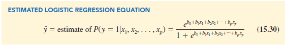
Here, y provides an estimate of the probability that y = 1 given a particular set of values for the independent variables.
Let us now return to the Simmons Stores example. The variables in the study are defined as follows:

Thus, we choose a logistic regression equation with two independent variables.
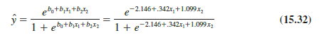
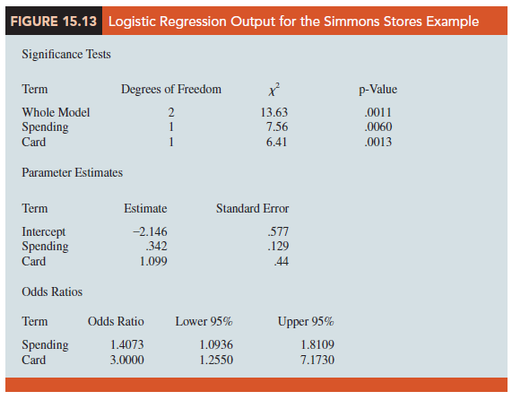
Using the sample data (see Table 15.11), we used statistical software to compute estimates of the model parameters b0, b1, and b2. Figure 15.13 displays output commonly provided by statistical software. We see that b0 = −2.146, b1 = .342, and b2 = 1.099.
Thus, the estimated logistic regression equation is
We can now use equation (15.32) to estimate the probability of using the coupon for a particular type of customer. For example, to estimate the probability of using the coupon for customers who spend $2000 annually and do not have a Simmons credit card, we substitute x1 = 2 and x2 = 0 into equation (15.32).
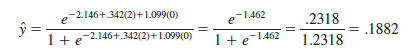
Thus, an estimate of the probability of using the coupon for this particular group of customers is approximately .19. Similarly, to estimate the probability of using the coupon for customers who spent $2000 last year and have a Simmons credit card, we substitute x1 = 2 and x2 = 1 into equation (15.32).
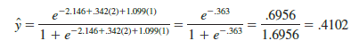
Thus, for this group of customers, the probability of using the coupon is approximately .41. It appears that the probability of using the coupon is much higher for customers with a Simmons credit card. Before reaching any conclusions, however, we need to assess the statistical significance of our model.
3. Testing for Significance
Testing for significance in logistic regression is similar to testing for significance in multiple regression. First we conduct a test for overall significance. For the Simmons Stores example, the hypotheses for the test of overall significance follow:
The test for overall significance is based upon the value of a 1 test statistic. If the null hypothesis is true, the sampling distribution of 1 follows a chi-square distribution with degrees of freedom equal to the number of independent variables in the model. While the calculations behind the computation of 1 is beyond the scope of the book, Figure 15.13 lists the value of 1 and its corresponding p-value in the Whole Model row of the Significance Tests table; we see that the value of 1 is 13.63, its degrees of freedom are 2, and its p-value is .0011. Thus, at any level of significance a > .0011, we would reject the null hypothesis and conclude that the overall model is significant.
If the 1 test shows an overall significance, another 1 test can be used to determine whether each of the individual independent variables is making a significant contribution to the overall model. For the independent variables xt, the hypotheses are
The test of significance for an independent variable is also based upon the value of a 1 test statistic. If the null hypothesis is true, the sampling distribution of 1 follows a chi-square distribution with one degree of freedom. The Spending and Card rows of the Significance Tests table of Figure 15.13 contain the values of 1 and their corresponding p-values test for the estimated coefficients. Suppose we use a = .05 to test for the significance of the independent variables in the Simmons model. For the independent variable Spending (x1) the x2 value is 7.56 and the corresponding p-value is .0060. Thus, at the .05 level of significance we can reject H0: β1 = 0. In a similar fashion we can also reject H0: β2 = 0 because the p-value corresponding to Card’s x2 = 6.41 is .0013. Hence, at the .05 level of significance, both independent variables are statistically significant.
4. Managerial Use
We described how to develop the estimated logistic regression equation and how to test it for significance. Let us now use it to make a decision recommendation concerning the Simmons Stores catalog promotion. For Simmons Stores, we already computed P( y = 1|x1 = 2, x2 = 1) = .4102 and P( y = 1|x1 = 2, x2 = 0) = .1881. These probabilities indicate that for customers with annual spending of $2000 the presence of a Simmons credit card increases the probability of using the coupon. In Table 15.12 we show estimated probabilities for values of annual spending ranging from $1000 to $7000 for both customers who have a Simmons credit card and customers who do not have a Simmons credit card. How can Simmons use this information to better target customers for the new promotion? Suppose Simmons wants to send the promotional catalog only to customers who have a .40 or higher probability of using the coupon. Using the estimated probabilities in Table 15.12, Simmons promotion strategy would be:
Customers who have a Simmons credit card: Send the catalog to every customer who spent $2000 or more last year.
Customers who do not have a Simmons credit card: Send the catalog to every customer who spent $6000 or more last year.
Looking at the estimated probabilities further, we see that the probability of using the coupon for customers who do not have a Simmons credit card but spend $5000 annually is .3922. Thus, Simmons may want to consider revising this strategy by including those customers who do not have a credit card, as long as they spent $5000 or more last year.

5. Interpreting the Logistic Regression Equation
Interpreting a regression equation involves relating the independent variables to the business question that the equation was developed to answer. With logistic regression, it is difficult to interpret the relation between the independent variables and the probability that y = 1 directly because the logistic regression equation is nonlinear. However, statisticians have shown that the relationship can be interpreted indirectly using a concept called the odds ratio.
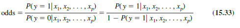
The odds in favor of an event occurring is defined as the probability the event will occur divided by the probability the event will not occur. In logistic regression the event of interest is always y = 1. Given a particular set of values for the independent variables, the odds in favor of y = 1 can be calculated as follows:
The odds ratio measures the impact on the odds of a one-unit increase in only one of the independent variables. The odds ratio is the odds that y = 1 given that one of the independent variables has been increased by one unit (odds1) divided by the odds that y = 1 given no change in the values for the independent variables (odds0).

For example, suppose we want to compare the odds of using the coupon for customers who spend $2000 annually and have a Simmons credit card (x1 = 2 and x2 = 1) to the odds of using the coupon for customers who spend $2000 annually and do not have a Simmons credit card (x1 = 2 and x2 = 0). We are interested in interpreting the effect of a one-unit increase in the independent variable x2. In this case
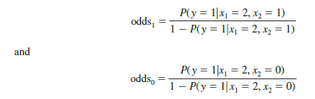
Previously we showed that an estimate of the probability that y = 1 given x1 = 2 and x2 = 1 is .4102, and an estimate of the probability that y = 1 given x1 = 2 and x2 = 0 is .1881. Thus,
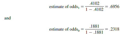
The estimated odds ratio is
![]()
Thus, we can conclude that the estimated odds in favor of using the coupon for customers who spent $2000 last year and have a Simmons credit card are 3 times greater than the estimated odds in favor of using the coupon for customers who spent $2000 last year and do not have a Simmons credit card.
The odds ratio for each independent variable is computed while holding all the other independent variables constant. But it does not matter what constant values are used for the other independent variables. For instance, if we computed the odds ratio for the Simmons credit card variable (x2) using $3000, instead of $2000, as the value for the annual spending variable (x1), we would still obtain the same value for the estimated odds ratio (3.00). Thus, we can conclude that the estimated odds of using the coupon for customers who have a Simmons credit card are 3 times greater than the estimated odds of using the coupon for customers who do not have a Simmons credit card.
The odds ratio is standard output for most statistical software packages. The Odds Ratios table in Figure 15.13 contains the estimated odds ratios for each of the independent variables. The estimated odds ratio for Spending (x1) is 1.4073 and the estimated odds ratio for Card (x2) is 3.0000. We already showed how to interpret the estimated odds ratio for the binary independent variable x2. Let us now consider the interpretation of the estimated odds ratio for the continuous independent variable x1.
The value of 1.4073 in the Odds Ratio column of the output tells us that the estimated odds in favor of using the coupon for customers who spent $3000 last year is 1.4073 times greater than the estimated odds in favor of using the coupon for customers who spent $2000 last year. Moreover, this interpretation is true for any one-unit change in x1. For instance, the estimated odds in favor of using the coupon for someone who spent $5000 last year is 1.4073 times greater than the odds in favor of using the coupon for a customer who spent $4000 last year. But suppose we are interested in the change in the odds for an increase of more than one unit for an independent variable. Note that x1 can range from 1 to 7. The odds ratio given by the output does not answer this question. To answer this question we must explore the relationship between the odds ratio and the regression coefficients.
A unique relationship exists between the odds ratio for a variable and its corresponding regression coefficient. For each independent variable in a logistic regression equation it can be shown that
![]()
To illustrate this relationship, consider the independent variable x1 in the Simmons example. The estimated odds ratio for x1 is
![]()
Similarly, the estimated odds ratio for x2 is
![]()
This relationship between the odds ratio and the coefficients of the independent variables makes it easy to compute estimated odds ratios once we develop estimates of the model parameters. Moreover, it also provides us with the ability to investigate changes in the odds ratio of more than or less than one unit for a continuous independent variable.
The odds ratio for an independent variable represents the change in the odds for a one- unit change in the independent variable holding all the other independent variables constant. Suppose that we want to consider the effect of a change of more than one unit, say c units. For instance, suppose in the Simmons example that we want to compare the odds of using the coupon for customers who spend $5000 annually (x1 = 5) to the odds of using the coupon for customers who spend $2000 annually (x1 = 2). In this case c = 5 – 2 = 3 and the corresponding estimated odds ratio is
![]()
This result indicates that the estimated odds of using the coupon for customers who spend $5000 annually is 2.79 times greater than the estimated odds of using the coupon for customers who spend $2000 annually. In other words, the estimated odds ratio for an increase of $3000 in annual spending is 2.79.
In general, the odds ratio enables us to compare the odds for two different events. If the value of the odds ratio is 1, the odds for both events are the same. Thus, if the independent variable we are considering (such as Simmons credit card status) has a positive impact on the probability of the event occurring, the corresponding odds ratio will be greater than 1.Most statistical software packages provide a confidence interval for the odds ratio. The Odds Ratio table in Figure 15.13 provides a 95% confidence interval for each of the odds ratios. For example, the point estimate of the odds ratio for x1 is 1.4073 and the 95% confidence interval is 1.0936 to 1.8109. Because the confidence interval does not contain the value of 1, we can conclude that x1 has a significant relationship with the estimated odds ratio. Similarly, the 95% confidence interval for the odds ratio for x2 is 1.2550 to 7.1730. Because this interval does not contain the value of 1, we can also conclude that x2 has a significant relationship with the odds ratio.
6. Logit Transformation
An interesting relationship can be observed between the odds in favor of y = 1 and the exponent for e in the logistic regression equation. It can be shown that
![]()
This equation shows that the natural logarithm of the odds in favor of y = 1 is a linear function of the independent variables. This linear function is called the logit. We will use the notation g(x1, x2, . . . , xp) to denote the logit.

Substituting g(x1, x2, . . . , xp) for β1 + β1×1 + β2×2 + . . . + bpxp in equation (15.27), we can write the logistic regression equation as
![]()
Once we estimate the parameters in the logistic regression equation, we can compute an estimate of the logit. Using tg(x1, x2, . . . , xp) to denote the estimated logit, we obtain
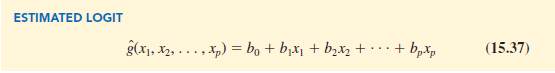
Thus, in terms of the estimated logit, the estimated regression equation is
For the Simmons Stores example, the estimated logit is
![]()
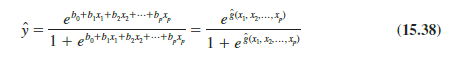
and the estimated regression equation is
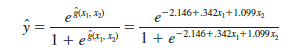
Thus, because of the unique relationship between the estimated logit and the estimated logistic regression equation, we can compute the estimated probabilities for Simmons Stores by dividing ![]()
Source: Anderson David R., Sweeney Dennis J., Williams Thomas A. (2019), Statistics for Business & Economics, Cengage Learning; 14th edition.
30 Aug 2021
31 Aug 2021
30 Aug 2021
30 Aug 2021
30 Aug 2021
30 Aug 2021