Sampling Distribution of x

In the previous section we said that the sample mean X is a random variable and its probability distribution is called the sampling distribution of X.

This section describes the properties of the sampling distribution of X. Just as with other probability distributions we studied, the sampling distribution of X has an expected value or mean, a standard deviation, and a characteristic shape or form. Let us begin by considering the mean of all possible X values, which is referred to as the expected value of X.

1. Expected Value of x

In the EAI sampling problem we saw that different simple random samples result in a vari­ety of values for the sample mean x. Because many different values of the random variable x are possible, we are often interested in the mean of all possible values of x that can be generated by the various simple random samples. The mean of the x random variable is the expected value of x. Let E(x) represent the expected value of x and m represent the mean of the population from which we are selecting a simple random sample. It can be shown that with simple random sampling, E(x) and m are equal.

This result shows that with simple random sampling, the expected value or mean of the sampling distribution of x is equal to the mean of the population. In Section 7.1 we saw that the mean annual salary for the population of EAI managers is μ = $71,800. Thus, according to equation (7.1), the mean of all possible sample means for the EAI study is also $71,800.

When the expected value of a point estimator equals the population parameter, we say the point estimator is unbiased. Thus, equation (7.1) shows that x is an unbiased estimator of the population mean μ.

2. Standard Deviation of x

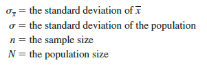
Let us define the standard deviation of the sampling distribution of x. We will use the following notation.

It can be shown that the formula for the standard deviation of x depends on whether the population is finite or infinite. The two formulas for the standard deviation of x follow.

In comparing the two formulas in (7.2), we see that the factor is required for the finite population case but not for the infinite population case. This factor is commonly referred to as the finite population correction factor. In many practical sampling situations, we find that the population involved, although finite, is “large,” whereas the sample size is relatively “small.” In such cases the finite population correction factor is close to 1. As a result, the difference between the values of the standard deviation of x for the finite and infinite population cases becomes negligible. Then,  becomes a good approximation to the standard deviation of X even though the population is finite. This observation leads to the following general guideline, or rule of thumb, for computing the standard deviation of X.

In cases where n/N > .05, the finite population version of formula (7.2) should be used in the computation of σ_x. Unless otherwise noted, throughout the text we will assume that the population size is “large,” n/N < .05, and expression (7.3) can be used to compute σ_x.

To compute σ_x, we need to know s, the standard deviation of the population. To further emphasize the difference between σ_x and σ, we refer to the standard deviation of X, σ_x, as the standard error of the mean. In general, the term standard error refers to the standard deviation of a point estimator. Later we will see that the value of the standard error of the mean is helpful in determining how far the sample mean may be from the population mean. Let us now return to the EAI example and compute the standard error of the mean associ­ated with simple random samples of 30 EAI managers.

In Section 7.1 we saw that the standard deviation of annual salary for the population of 2500 EAI managers is s = 4000. In this case, the population is finite, with N = 2500. However, with a sample size of 30, we have n/N = 30/2500 = .012. Because the sample size is less than 5% of the population size, we can ignore the finite population correction factor and use equation (7.3) to compute the standard error.

3. Form of the Sampling Distribution of x

The preceding results concerning the expected value and standard deviation for the sampling distribution of x are applicable for any population. The final step in identifying the characteristics of the sampling distribution of x is to determine the form or shape of the sampling distribution. We will consider two cases: (1) The population has a normal distribution; and (2) the population does not have a normal distribution.

Population has a Normal Distribution In many situations it is reasonable to assume that the population from which we are selecting a random sample has a normal, or nearly nor­mal, distribution. When the population has a normal distribution, the sampling distribution of x is normally distributed for any sample size.

Population does not have a Normal Distribution When the population from which we are selecting a random sample does not have a normal distribution, the central limit theorem is helpful in identifying the shape of the sampling distribution of x.

A statement of the central limit theorem as it applies to the sampling distribution of x follows.

Figure 7.3 shows how the central limit theorem works for three different populations; each column refers to one of the populations. The top panel of the figure shows that none of the populations are normally distributed. Population I follows a uniform distribution. Population II is often called the rabbit-eared distribution. It is symmetric, but the more likely values fall in the tails of the distribution. Population III is shaped like the exponential distribution; it is skewed to the right.

The bottom three panels of Figure 7.3 show the shape of the sampling distribution for samples of size n = 2, n = 5, and n = 30. When the sample size is 2, we see that the shape of each sampling distribution is different from the shape of the corresponding population distribution. For samples of size 5, we see that the shapes of the sampling dis­tributions for populations I and II begin to look similar to the shape of a normal distribu­tion. Even though the shape of the sampling distribution for population III begins to look similar to the shape of a normal distribution, some skewness to the right is still present. Finally, for samples of size 30, the shapes of each of the three sampling distributions are approximately normal.

From a practitioner standpoint, we often want to know how large the sample size needs to be before the central limit theorem applies and we can assume that the shape of the sampling distribution is approximately normal. Statistical researchers have investig­ated this question by studying the sampling distribution of X for a variety of populations and a variety of sample sizes. General statistical practice is to assume that, for most applications, the sampling distribution of X can be approximated by a normal distribution whenever the sample is size 30 or more. In cases where the population is highly skewed or outliers are present, samples of size 50 may be needed. Finally, if the population is discrete, the sample size needed for a normal approximation often depends on the popu­lation proportion. We say more about this issue when we discuss the sampling distribu­tion of p in Section 7.6.

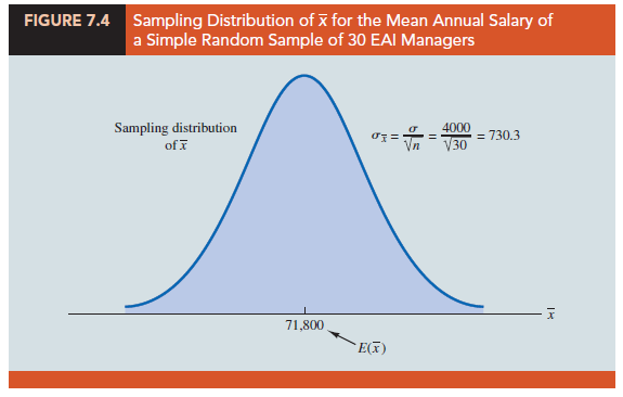
4. Sampling Distribution of x for the EAI Problem

Let us return to the EAI problem where we previously showed that E(X) = $71,800 and s_x = 730.3. At this point, we do not have any information about the population dis­tribution; it may or may not be normally distributed. If the population has a normal distribution, the sampling distribution of X is normally distributed. If the population does not have a normal distribution, the simple random sample of 30 managers and the central limit theorem enable us to conclude that the sampling distribution of X can be approx­imated by a normal distribution. In either case, we are comfortable proceeding with the conclusion that the sampling distribution of X can be described by the normal distribution shown in Figure 7.4.

5. Practical Value of the Sampling Distribution of x

Whenever a simple random sample is selected and the value of the sample mean is used to estimate the value of the population mean m, we cannot expect the sample mean to exactly equal the population mean. The practical reason we are interested in the sampling distri­bution of X is that it can be used to provide probability information about the difference between the sample mean and the population mean. To demonstrate this use, let us return to the EAI problem.

Suppose the personnel director believes the sample mean will be an acceptable estimate of the population mean if the sample mean is within $500 of the population mean. However, it is not possible to guarantee that the sample mean will be within $500 of the population mean. Indeed, Table 7.5 and Figure 7.1 show that some of the 500 sample means differed by more than $2000 from the population mean. So we must think of the personnel director’s request in probability terms. That is, the personnel director is concerned with the following question: What is the probability that the sample mean computed using a simple random sample of 30 EAI managers will be within $500 of the population mean?

Because we have identified the properties of the sampling distribution of X (see Figure 7.4), we will use this distribution to answer the probability question. Refer to the sampling distribution of X shown again in Figure 7.5. With a population mean of $71,800, the personnel director wants to know the probability that X is between $71,300 and $72,300. This probability is given by the darkly shaded area of the sampling distribution shown in Figure 7.5. Because the sampling distribution is normally distributed, with mean 71,800 and standard error of the mean 730.3, we can use the standard normal probability table to find the area or probability.

We first calculate the z value at the upper endpoint of the interval (72,300) and use the table to find the area under the curve to the left of that point (left tail area). Then we com­pute the z value at the lower endpoint of the interval (71,300) and use the table to find the area under the curve to the left of that point (another left tail area). Subtracting the second tail area from the first gives us the desired probability.

At X = 72,300, we have

Referring to the standard normal probability table, we find a cumulative probability (area to the left of z = .68) of .7517.

The preceding computations show that a simple random sample of 30 EAI managers has a .5034 probability of providing a sample mean X that is within $500 of the popula­tion mean. Thus, there is a 1 – .5034 = .4966 probability that the difference between X and m = $71,800 will be more than $500. In other words, a simple random sample of 30 EAI managers has roughly a 50-50 chance of providing a sample mean within the allowable $500. Perhaps a larger sample size should be considered. Let us explore this possibility by considering the relationship between the sample size and the sampling distribution of X.

6. Relationship Between the Sample Size and the Sampling Distribution of x

Suppose that in the EAI sampling problem we select a simple random sample of 100 EAI managers instead of the 30 originally considered. Intuitively, it would seem that with more data provided by the larger sample size, the sample mean based on n = 100 should provide a better estimate of the population mean than the sample mean based on n = 30. To see how much better, let us consider the relationship between the sample size and the sampling distribution of X.

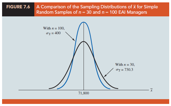
First note that E(x) = m regardless of the sample size. Thus, the mean of all possible values of X is equal to the population mean m regardless of the sample size n. However, note that the standard error of the mean, s_X = s/yn, is related to the square root of the sample size. Whenever the sample size is increased, the standard error of the mean s_X decreases. With n = 30, the standard error of the mean for the EAI problem is 730.3. However, with the increase in the sample size to n = 100, the standard error of the mean is decreased to

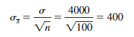
The sampling distributions of X with n = 30 and n = 100 are shown in Figure 7.6. Because the sampling distribution with n = 100 has a smaller standard error, the values of X have less variation and tend to be closer to the population mean than the values of X with n = 30.

We can use the sampling distribution of X for the case with n = 100 to compute the probability that a simple random sample of 100 EAI managers will provide a sample mean that is within $500 of the population mean. Because the sampling distribution is normal, with mean 71,800 and standard error of the mean 400, we can use the standard normal probability table to find the area or probability.

At X = 72,300 (see Figure 7.7), we have

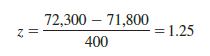
Referring to the standard normal probability table, we find a cumulative probability corresponding to z = 1.25 of .8944.

The cumulative probability corresponding to z = -1.25 is .1056. Therefore, P(71,300 ≤ x ≤ 72,300) = P(z ≤ 1.25) – P(z ≤ -1.25) = .8944 – .1056 = .7888. Thus, by increas­ing the sample size from 30 to 100 EAI managers, we increase the probability of obtaining a sample mean within $500 of the population mean from .5034 to .7888.

The important point in this discussion is that as the sample size is increased, the standard error of the mean decreases. As a result, the larger sample size provides a higher probability that the sample mean is within a specified distance of the population mean.

Source:  Anderson David R., Sweeney Dennis J., Williams Thomas A. (2019), Statistics for Business & Economics, Cengage Learning; 14th edition.